Chapter 6 Sampling Distributions
In this chapter, we’ll cover three ideas/questions.
- What are inferential statistics and the logic behind them
- What the underlying distribution of all hypothetical sample estimates is known as the sampling distribution, and it constitutes the third of the three important distributions.
- Several important implications follow from an understanding of the sampling distribution as a normal distribution and from the central limit theorem
Spoken about a bit before in the other chapter, we have both sample statistics like \(\bar{X}\) and population parameters \(\mu\).
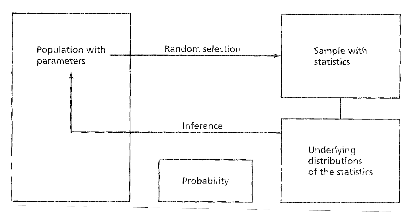
The idea of how frequentist inferential statistics is as follows. Samples must be selected randomly in order to make appropopriate inferences about the parent population. Sample estimates must be compared to an underlying distributionof estimates of all other hypothetical samples of that same sizefrom the parent population. Based on this comparison and the associated probability of obtaining certain outcomes, inferences can be made about population parameters.
Sampling
It’s important to note that there are three different distributions that we typically talk about. Two you should be familiar with – the populatation and the sample. The third is the sampling distribution which is a distribution of sample means. The sampling distribution of the mean is generated by considering all possible sample means of a given sample size.
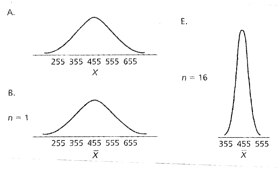
As is demonstratd from the image below, in A we can see there is some sort of distribution, then with one sample (notice the \(\bar{X}\)), we now have one wide sample.
As we increase that to \(N = 16\), the sampling distribution becomes more narrow.
This narrowing is reflective of the idea we are coming in on the true value of the population via our random sampling.
The central limit theorem states that as the sample size \(n\) increases, the sampling distribution of the mean for simple random samples of \(n\) cases, taken from a population with a mean equal to \(\mu\) and a finite variance equal to \(\sigma^2\), approximates a normal distribution. From this, three points follow:
1.The shape of the sampling distribution is normal 2. The mean of the sampling distribution is \(\mu\) 3. The standard deviation of the sampling distribution, or standard error of the mean, is \[\frac{\sigma}{\sqrt{n}}= \sigma_\bar{X}\]
Several important implications follow from an understanding of the sampling distribution as a normal distribution and from the central limit theorem.
Because we know the mean and standard error, we can calculate the probability of selecting a random sample mean that is at or more extreme than a particular value on the distribution.
\[z = \frac{\bar{X}-\mu}{\sigma_\bar{X}}\]
We can appeal to the table of z scores on the standard normal distribution to find the probability.
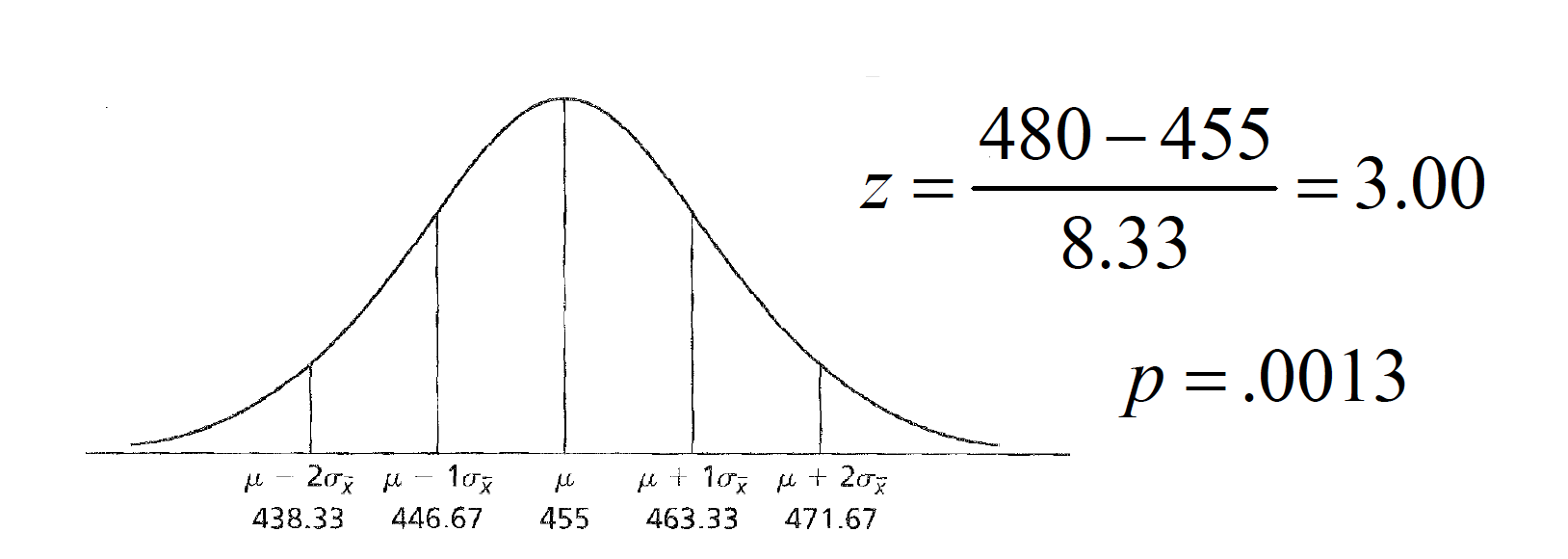
For example, consider a sampling distribution of SAT scores with a mean of 455 and a standard error of 8.33. This standard error was generated with \(n\)= 144 and \(\sigma\)= 100.
So if you wanted to find the liklihood of finding as ample mean equal to or more than extreme of 480, we would plug it into the follow equation. \[z = \frac{480 - 455}{8.33} = 3.00\] And if we look that up a table of z distributions, we got a probability of \(p=.0013\).
Sampling
Because we know the mean and standard error, we can calculate the probability of selecting a random sample mean that is at or more extreme than a particular value on the distribution.
As sample size (\(n\)) increases, the variability of the sampling distribution (\(\sigma_\bar{X}\)) decreases.
Even when the parent population is not normally distributed, the sampling distribution becomes normal as sample size (n) increases.
You can see this demonstrated in THIS LINK.