Chapter 2 Introduction to R
Before starting out, it’s worth mentioning that R has a steep learning curve compared to other statistical softwares. While there are tons of blog posts as to why you should learn R, I will keep my list quick so if you get discouraged at any point, you can come back to this list and get re-inspired before R starts paying you back.
- The R community is fantastic, check out #rstats on Twitter as well as everyone affiliated with the tidyVerse
- R will always be free because the people behind it believe in open source principles.
- Time spent learning R is time spent learning how computers work. If you learn about R, you are also learning computer programming. Time spent in something like SPSS or SAS does not easily transfer to other programs.
- On r-jobs.com the way they decide to split jobs is jobs that make above and below $100,000.
- R is your ticket out of academia, if you need it. It’s also insane to think people would learn so much about statistics, the hardest part about becoming a data scientist, without learning the software to get you in the door.
- When you make analyses and graphs in R they are very easy to reproduce. You just press ‘Run’ again.
- If you do your data cleaning in R, then each step is documented. There is less chance for human error.
- It makes gorgeous graphs.
- There are a lot of ways that R integrates into other software. This book is written in bookdown, my website is written in blogdown, you can also make interactive data applications.
- It’s kind of fun.
2.1 Getting Started
Since this book is about statistics and R, the introduction to all things R is a bit shorter than other guides. If you need help, find a friend (or email the author of this book) and they will get you started. The first things you need to do is download R from CRAN, then get the latest version of RStudio. RStudio is an IDE that makes working in R a lot easier. If you use R without RStudio, you are basically a masochist.
Once you have that, you can start to play around with this.
2.2 A Note on Setting the Working Directory
At the end a long writing session you normally have to find a place to save that journal article you are working on. You do this by clicking ‘Save As’ then finding where to stick it and what to call it. If you are programming you need to do this entire act of picking where you are working right away by saving your script (the what) and setting your working directory (the where). After running a couple of “teach yourself R” sessions, I have found that this concept is one of the most tedious parts of starting to learn R, but once you are over this hump, the others will not feel as bad. While these instructions below are meant to be comprehensive, it’s much easier to learn this part of the process with someone walking you through the steps.
When you first open R, it’s good to get in the habit of seeing where your working directory is set to. If RStudio is set on it’s default settings, there should be a little line right above the console just like the image below.
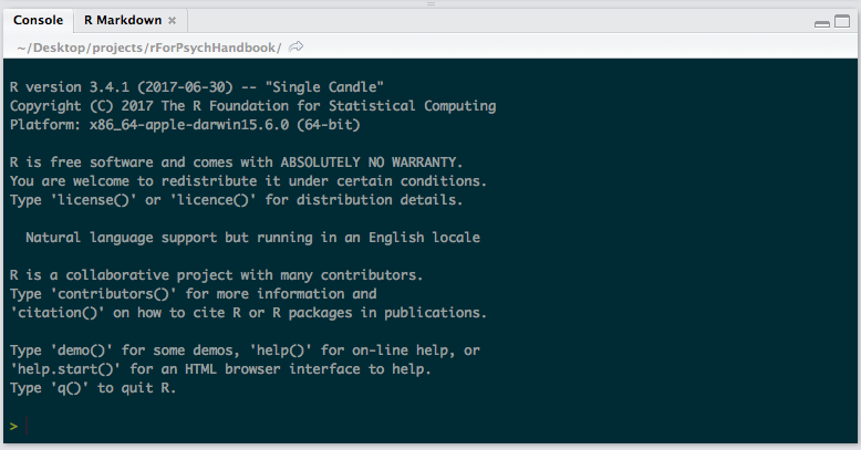
Current Working Directory Location
This whole book exists in a folder that lives in the projects folder on my Desktop. If you’re not familiar with how your computer is set up, it’s worth checking out an explanation or having someone walk you through the hierarchy your computer’s directories.
Once you have an basic understanding of this, you can find where you are in R by using the getwd() function.
If you need to change your working directory at any point, the function is setwd().
While it might seem a bit tedious to have to think about things like this right away, by setting up analysis projects in a clean, and organized way you are going to be saving yourself hours in the future.
So with that, open up a new R script, and for your first line set your working directory to a folder where you are going to want to work out of.
2.3 The Basics
With this script set up, we can now start to play around with R! This chapter covers a few basic things:
- The rationale behind to writing scripts and code
- R as Calculator
- Data Structures
- Manipulating Data
- Tons of functions
- Whirlwind tour of R for psychologists
The goals of this chapter are to:
- Learn Basics of R and RStudio
- Practice concepts with simple examples
- Familiarize with vast array of functions
- Have vocabulary and “R” way to think about problem solving
2.4 R as Calculator
The Console of R is where all the action happens. You can use it just like you would use a calculator. Try to do some basic math operations in it.
## [1] 4## [1] 3## [1] 2.5## [1] 1800## [1] 9## [1] TRUE## [1] FALSEYou don’t always want to print your output and retype it in. The idea of being a good programmer is to be very lazy (efficient).
One of the best ways to be efficient when programming is to save variables to objects.
Below is some example code that uses the <- operator to assign some math to an object.
After you assign it to an object, you can then manipulate it like you would any other number.
## [1] 36After running these two lines of code, notice what has popped up in your environment in RStudio!
You should see that you now have any object in the Environment called foo.
In addition to saving single values to objects, you can also store a collection of values. Below we use an example that might have a bit more meaning, the below stores what could be some data into an object that represents what it might be.
The way that the line above works is that we use the c() function (c for concatenate) to group together a bunch of the same type of data (numbers) into a vector.
Once we have everything concatenated and stored into an object, we can then manipulate all the numbers in the object just like we did above with a single number.
For example, we could multiply all the numbers by three.
## [1] 6 3 12 15 18 21 9 6 12 15 9Or maybe we realized that our inputs were wrong and we need to shave off two years off of each of the entries.
## [1] 0 -1 2 3 4 5 1 0 2 3 1Or perhaps we want to find out which of our pieces of data (and other data associated with that observation) are less than 2.
## [1] FALSE TRUE FALSE FALSE FALSE FALSE FALSE FALSE FALSE FALSE FALSEAny sort of mathematical operation can be performed on a vector! In addition to treating it like a mathematical operation, we can also run functions on objects. By looking at the name of each function and it’s output, take a guess at what each of the below functions does.
## [1] 3.818182## [1] 1.834022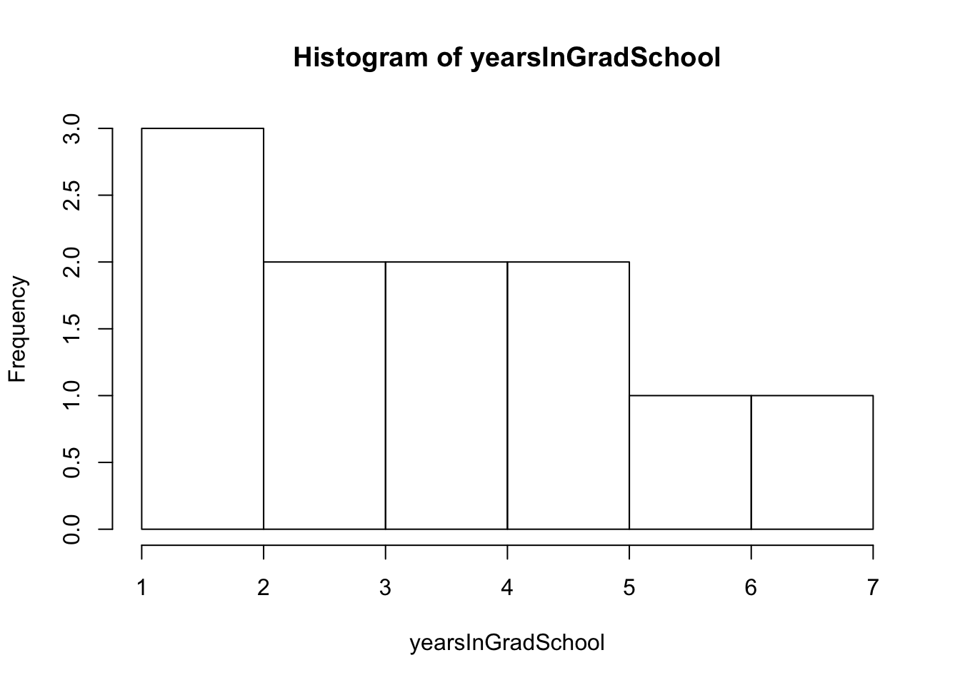
##              [,1]
##  [1,] -0.99136319
##  [2,] -1.53661295
##  [3,]  0.09913632
##  [4,]  0.64438608
##  [5,]  1.18963583
##  [6,]  1.73488559
##  [7,] -0.44611344
##  [8,] -0.99136319
##  [9,]  0.09913632
## [10,]  0.64438608
## [11,] -0.44611344
## attr(,"scaled:center")
## [1] 3.818182
## attr(,"scaled:scale")
## [1] 1.834022## [1] 1 7## [1] 1## [1] "numeric"## num [1:11] 2 1 4 5 6 7 3 2 4 5 ...## Min. 1st Qu. Median Mean 3rd Qu. Max.
## 1.000 2.500 4.000 3.818 5.000 7.000Often working with data, we don’t want to just play with one group of numbers. Most of the time we are trying to compare diffrent observations in psychology. If we then create two vectors (one of which we have already made!) and then combine them together into a data frame, we have something sort of looking like a spreadsheet.
yearsInGradSchool <- c(2,1,4,5,6,7,3,2,4,5,3)
classesTaken <- c(5,2,5,7,9,9,2,8,4,7,2)
gradData <- data.frame(yearsInGradSchool,classesTaken)
gradData
## yearsInGradSchool classesTaken
## 1 2 5
## 2 1 2
## 3 4 5
## 4 5 7
## 5 6 9
## 6 7 9
## 7 3 2
## 8 2 8
## 9 4 4
## 10 5 7
## 11 3 2Now if we wanted to use something like R’s correlation function we could just pass in the two objects that we have like this and get a correlation value.
## [1] 0.6763509But often our data will be saved in data frames and we need to be able to access one of our vectors inside our data frame.
To access a piece of information in a data frame we use the $ operator.
## [1] 2 1 4 5 6 7 3 2 4 5 3Running the above code will print out the vector called yearsInGradSchool from the data frame gradData.
Using this form, we can then use this with the correrlation function.
## [1] 0.6763509In addition to just getting numeric output, we also want to be able to look at our data. Take a look at the code below and try to figure out what the function call is, as well as what each argument (or thing you pass to a function) does.
plot(yearsInGradSchool,classesTaken,
     data = gradData,
     main = "My Plot",
     xlab = "Years in Grad School",
     ylab = "Classes Taken")
## Warning in plot.window(...): "data" is not a graphical parameter## Warning in plot.xy(xy, type, ...): "data" is not a graphical parameter## Warning in axis(side = side, at = at, labels = labels, ...): "data" is not
## a graphical parameter
## Warning in axis(side = side, at = at, labels = labels, ...): "data" is not
## a graphical parameter## Warning in box(...): "data" is not a graphical parameter## Warning in title(...): "data" is not a graphical parameter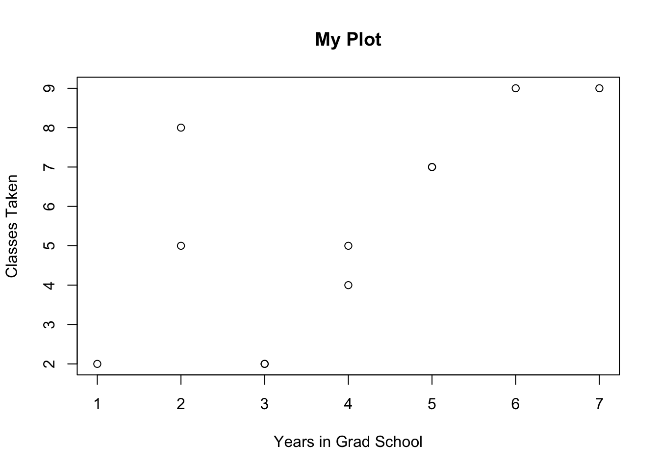
If you are having a hard time understanding arguments, one thing that might help to think about is that each argument is like a click in a software program like SPSS.
Imagine you want to make the same plot with this data in SSPSS, what would you do?
The first thing you would do is to go to the top of the bar and find the Plot function and click it.
This is the same as typing out plot() in R.
Then you would have to tell that new pop up screen what two variables you want to plot and click on the related variables.
Dragging and dropping those variables into your plot builder is the same as just typing out the variables you want.
Laslty you want to put names on your axes and a title on your plot.
The same logic would follow.
We’ll explore these ideas a bit more in the next section.
2.5 Data Exploration
## 'data.frame':    150 obs. of  5 variables:
##  $ Sepal.Length: num  5.1 4.9 4.7 4.6 5 5.4 4.6 5 4.4 4.9 ...
##  $ Sepal.Width : num  3.5 3 3.2 3.1 3.6 3.9 3.4 3.4 2.9 3.1 ...
##  $ Petal.Length: num  1.4 1.4 1.3 1.5 1.4 1.7 1.4 1.5 1.4 1.5 ...
##  $ Petal.Width : num  0.2 0.2 0.2 0.2 0.2 0.4 0.3 0.2 0.2 0.1 ...
## $ Species : Factor w/ 3 levels "setosa","versicolor",..: 1 1 1 1 1 1 1 1 1 1 ...## [1] "data.frame"## Sepal.Length Sepal.Width Petal.Length Petal.Width
## Min. :4.300 Min. :2.000 Min. :1.000 Min. :0.100
## 1st Qu.:5.100 1st Qu.:2.800 1st Qu.:1.600 1st Qu.:0.300
## Median :5.800 Median :3.000 Median :4.350 Median :1.300
## Mean :5.843 Mean :3.057 Mean :3.758 Mean :1.199
## 3rd Qu.:6.400 3rd Qu.:3.300 3rd Qu.:5.100 3rd Qu.:1.800
## Max. :7.900 Max. :4.400 Max. :6.900 Max. :2.500
## Species
## setosa :50
## versicolor:50
## virginica :50
##
##
## Accessing individual ‘columns’ is done with the $ operator
##   [1] 5.1 4.9 4.7 4.6 5.0 5.4 4.6 5.0 4.4 4.9 5.4 4.8 4.8 4.3 5.8 5.7 5.4
##  [18] 5.1 5.7 5.1 5.4 5.1 4.6 5.1 4.8 5.0 5.0 5.2 5.2 4.7 4.8 5.4 5.2 5.5
##  [35] 4.9 5.0 5.5 4.9 4.4 5.1 5.0 4.5 4.4 5.0 5.1 4.8 5.1 4.6 5.3 5.0 7.0
##  [52] 6.4 6.9 5.5 6.5 5.7 6.3 4.9 6.6 5.2 5.0 5.9 6.0 6.1 5.6 6.7 5.6 5.8
##  [69] 6.2 5.6 5.9 6.1 6.3 6.1 6.4 6.6 6.8 6.7 6.0 5.7 5.5 5.5 5.8 6.0 5.4
##  [86] 6.0 6.7 6.3 5.6 5.5 5.5 6.1 5.8 5.0 5.6 5.7 5.7 6.2 5.1 5.7 6.3 5.8
## [103] 7.1 6.3 6.5 7.6 4.9 7.3 6.7 7.2 6.5 6.4 6.8 5.7 5.8 6.4 6.5 7.7 7.7
## [120] 6.0 6.9 5.6 7.7 6.3 6.7 7.2 6.2 6.1 6.4 7.2 7.4 7.9 6.4 6.3 6.1 7.7
## [137] 6.3 6.4 6.0 6.9 6.7 6.9 5.8 6.8 6.7 6.7 6.3 6.5 6.2 5.9
Can you use this to plot the different numeric values against each other?
What would the follow commands do?
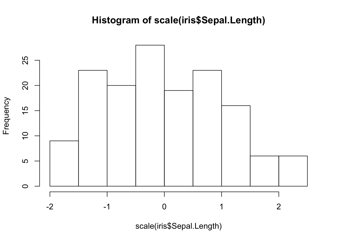
2.6 Indexing
Let’s combine logical indexing with creating new objects.
What do the follow commands do? Why?
## [1] 5.1## Sepal.Length Sepal.Width Petal.Length Petal.Width Species
## 2 4.9 3 1.4 0.2 setosa
## Sepal.Length.scale
## 2 -1.1392## [1] setosa setosa setosa setosa setosa setosa
## [7] setosa setosa setosa setosa setosa setosa
## [13] setosa setosa setosa setosa setosa setosa
## [19] setosa setosa setosa setosa setosa setosa
## [25] setosa setosa setosa setosa setosa setosa
## [31] setosa setosa setosa setosa setosa setosa
## [37] setosa setosa setosa setosa setosa setosa
## [43] setosa setosa setosa setosa setosa setosa
## [49] setosa setosa versicolor versicolor versicolor versicolor
## [55] versicolor versicolor versicolor versicolor versicolor versicolor
## [61] versicolor versicolor versicolor versicolor versicolor versicolor
## [67] versicolor versicolor versicolor versicolor versicolor versicolor
## [73] versicolor versicolor versicolor versicolor versicolor versicolor
## [79] versicolor versicolor versicolor versicolor versicolor versicolor
## [85] versicolor versicolor versicolor versicolor versicolor versicolor
## [91] versicolor versicolor versicolor versicolor versicolor versicolor
## [97] versicolor versicolor versicolor versicolor virginica virginica
## [103] virginica virginica virginica virginica virginica virginica
## [109] virginica virginica virginica virginica virginica virginica
## [115] virginica virginica virginica virginica virginica virginica
## [121] virginica virginica virginica virginica virginica virginica
## [127] virginica virginica virginica virginica virginica virginica
## [133] virginica virginica virginica virginica virginica virginica
## [139] virginica virginica virginica virginica virginica virginica
## [145] virginica virginica virginica virginica virginica virginica
## Levels: setosa versicolor virginica## Sepal.Length Sepal.Width Petal.Length Petal.Width Species
## 2 4.9 3.0 1.4 0.2 setosa
## 3 4.7 3.2 1.3 0.2 setosa
## 4 4.6 3.1 1.5 0.2 setosa
## 7 4.6 3.4 1.4 0.3 setosa
## 9 4.4 2.9 1.4 0.2 setosa
## 10 4.9 3.1 1.5 0.1 setosa
## 12 4.8 3.4 1.6 0.2 setosa
## 13 4.8 3.0 1.4 0.1 setosa
## 14 4.3 3.0 1.1 0.1 setosa
## 23 4.6 3.6 1.0 0.2 setosa
## 25 4.8 3.4 1.9 0.2 setosa
## 30 4.7 3.2 1.6 0.2 setosa
## 31 4.8 3.1 1.6 0.2 setosa
## 35 4.9 3.1 1.5 0.2 setosa
## 38 4.9 3.6 1.4 0.1 setosa
## 39 4.4 3.0 1.3 0.2 setosa
## 42 4.5 2.3 1.3 0.3 setosa
## 43 4.4 3.2 1.3 0.2 setosa
## 46 4.8 3.0 1.4 0.3 setosa
## 48 4.6 3.2 1.4 0.2 setosa
## 58 4.9 2.4 3.3 1.0 versicolor
## 107 4.9 2.5 4.5 1.7 virginica
## Sepal.Length.scale
## 2 -1.139200
## 3 -1.380727
## 4 -1.501490
## 7 -1.501490
## 9 -1.743017
## 10 -1.139200
## 12 -1.259964
## 13 -1.259964
## 14 -1.863780
## 23 -1.501490
## 25 -1.259964
## 30 -1.380727
## 31 -1.259964
## 35 -1.139200
## 38 -1.139200
## 39 -1.743017
## 42 -1.622254
## 43 -1.743017
## 46 -1.259964
## 48 -1.501490
## 58 -1.139200
## 107 -1.139200## Sepal.Length Sepal.Width Petal.Length Petal.Width
## 1 5.1 3.5 1.4 0.2
## 2 4.9 3.0 1.4 0.2
## 3 4.7 3.2 1.3 0.2
## 4 4.6 3.1 1.5 0.2
## 5 5.0 3.6 1.4 0.2
## 6 5.4 3.9 1.7 0.4
## 7 4.6 3.4 1.4 0.3
## 8 5.0 3.4 1.5 0.2
## 9 4.4 2.9 1.4 0.2
## 10 4.9 3.1 1.5 0.1
## 11 5.4 3.7 1.5 0.2
## 12 4.8 3.4 1.6 0.2
## 13 4.8 3.0 1.4 0.1
## 14 4.3 3.0 1.1 0.1
## 15 5.8 4.0 1.2 0.2
## 16 5.7 4.4 1.5 0.4
## 17 5.4 3.9 1.3 0.4
## 18 5.1 3.5 1.4 0.3
## 19 5.7 3.8 1.7 0.3
## 20 5.1 3.8 1.5 0.3
## 21 5.4 3.4 1.7 0.2
## 22 5.1 3.7 1.5 0.4
## 23 4.6 3.6 1.0 0.2
## 24 5.1 3.3 1.7 0.5
## 25 4.8 3.4 1.9 0.2
## 26 5.0 3.0 1.6 0.2
## 27 5.0 3.4 1.6 0.4
## 28 5.2 3.5 1.5 0.2
## 29 5.2 3.4 1.4 0.2
## 30 4.7 3.2 1.6 0.2
## 31 4.8 3.1 1.6 0.2
## 32 5.4 3.4 1.5 0.4
## 33 5.2 4.1 1.5 0.1
## 34 5.5 4.2 1.4 0.2
## 35 4.9 3.1 1.5 0.2
## 36 5.0 3.2 1.2 0.2
## 37 5.5 3.5 1.3 0.2
## 38 4.9 3.6 1.4 0.1
## 39 4.4 3.0 1.3 0.2
## 40 5.1 3.4 1.5 0.2
## 41 5.0 3.5 1.3 0.3
## 42 4.5 2.3 1.3 0.3
## 43 4.4 3.2 1.3 0.2
## 44 5.0 3.5 1.6 0.6
## 45 5.1 3.8 1.9 0.4
## 46 4.8 3.0 1.4 0.3
## 47 5.1 3.8 1.6 0.2
## 48 4.6 3.2 1.4 0.2
## 49 5.3 3.7 1.5 0.2
## 50 5.0 3.3 1.4 0.2
## 51 7.0 3.2 4.7 1.4
## 52 6.4 3.2 4.5 1.5
## 53 6.9 3.1 4.9 1.5
## 54 5.5 2.3 4.0 1.3
## 55 6.5 2.8 4.6 1.5
## 56 5.7 2.8 4.5 1.3
## 57 6.3 3.3 4.7 1.6
## 58 4.9 2.4 3.3 1.0
## 59 6.6 2.9 4.6 1.3
## 60 5.2 2.7 3.9 1.4
## 61 5.0 2.0 3.5 1.0
## 62 5.9 3.0 4.2 1.5
## 63 6.0 2.2 4.0 1.0
## 64 6.1 2.9 4.7 1.4
## 65 5.6 2.9 3.6 1.3
## 66 6.7 3.1 4.4 1.4
## 67 5.6 3.0 4.5 1.5
## 68 5.8 2.7 4.1 1.0
## 69 6.2 2.2 4.5 1.5
## 70 5.6 2.5 3.9 1.1
## 71 5.9 3.2 4.8 1.8
## 72 6.1 2.8 4.0 1.3
## 73 6.3 2.5 4.9 1.5
## 74 6.1 2.8 4.7 1.2
## 75 6.4 2.9 4.3 1.3
## 76 6.6 3.0 4.4 1.4
## 77 6.8 2.8 4.8 1.4
## 78 6.7 3.0 5.0 1.7
## 79 6.0 2.9 4.5 1.5
## 80 5.7 2.6 3.5 1.0
## 81 5.5 2.4 3.8 1.1
## 82 5.5 2.4 3.7 1.0
## 83 5.8 2.7 3.9 1.2
## 84 6.0 2.7 5.1 1.6
## 85 5.4 3.0 4.5 1.5
## 86 6.0 3.4 4.5 1.6
## 87 6.7 3.1 4.7 1.5
## 88 6.3 2.3 4.4 1.3
## 89 5.6 3.0 4.1 1.3
## 90 5.5 2.5 4.0 1.3
## 91 5.5 2.6 4.4 1.2
## 92 6.1 3.0 4.6 1.4
## 93 5.8 2.6 4.0 1.2
## 94 5.0 2.3 3.3 1.0
## 95 5.6 2.7 4.2 1.3
## 96 5.7 3.0 4.2 1.2
## 97 5.7 2.9 4.2 1.3
## 98 6.2 2.9 4.3 1.3
## 99 5.1 2.5 3.0 1.1
## 100 5.7 2.8 4.1 1.3
## 101 6.3 3.3 6.0 2.5
## 102 5.8 2.7 5.1 1.9
## 103 7.1 3.0 5.9 2.1
## 104 6.3 2.9 5.6 1.8
## 105 6.5 3.0 5.8 2.2
## 106 7.6 3.0 6.6 2.1
## 107 4.9 2.5 4.5 1.7
## 108 7.3 2.9 6.3 1.8
## 109 6.7 2.5 5.8 1.8
## 110 7.2 3.6 6.1 2.5
## 111 6.5 3.2 5.1 2.0
## 112 6.4 2.7 5.3 1.9
## 113 6.8 3.0 5.5 2.1
## 114 5.7 2.5 5.0 2.0
## 115 5.8 2.8 5.1 2.4
## 116 6.4 3.2 5.3 2.3
## 117 6.5 3.0 5.5 1.8
## 118 7.7 3.8 6.7 2.2
## 119 7.7 2.6 6.9 2.3
## 120 6.0 2.2 5.0 1.5
## 121 6.9 3.2 5.7 2.3
## 122 5.6 2.8 4.9 2.0
## 123 7.7 2.8 6.7 2.0
## 124 6.3 2.7 4.9 1.8
## 125 6.7 3.3 5.7 2.1
## 126 7.2 3.2 6.0 1.8
## 127 6.2 2.8 4.8 1.8
## 128 6.1 3.0 4.9 1.8
## 129 6.4 2.8 5.6 2.1
## 130 7.2 3.0 5.8 1.6
## 131 7.4 2.8 6.1 1.9
## 132 7.9 3.8 6.4 2.0
## 133 6.4 2.8 5.6 2.2
## 134 6.3 2.8 5.1 1.5
## 135 6.1 2.6 5.6 1.4
## 136 7.7 3.0 6.1 2.3
## 137 6.3 3.4 5.6 2.4
## 138 6.4 3.1 5.5 1.8
## 139 6.0 3.0 4.8 1.8
## 140 6.9 3.1 5.4 2.1
## 141 6.7 3.1 5.6 2.4
## 142 6.9 3.1 5.1 2.3
## 143 5.8 2.7 5.1 1.9
## 144 6.8 3.2 5.9 2.3
## 145 6.7 3.3 5.7 2.5
## 146 6.7 3.0 5.2 2.3
## 147 6.3 2.5 5.0 1.9
## 148 6.5 3.0 5.2 2.0
## 149 6.2 3.4 5.4 2.3
## 150 5.9 3.0 5.1 1.8## Sepal.Length Sepal.Width Petal.Length Species
## 1 5.1 3.5 1.4 setosa
## 2 4.9 3.0 1.4 setosa
## 3 4.7 3.2 1.3 setosa
## 4 4.6 3.1 1.5 setosa
## 5 5.0 3.6 1.4 setosa
## 6 5.4 3.9 1.7 setosa
## 8 5.0 3.4 1.5 setosaThis could be an entire lecture by itself!!!
2.7 Whirlwind Tour of R
R’s power comes in the fact that you download packages to put on top of base R
- Turning Data tables into already formatted APA Latex Tables (stargazer, xtable)
- Creating Publication Quality Graphs (ggplot2)
- Text manipulation (stringr)
- Exploring data and not making chart after chart after chart (psych)
- Every statistical test you could want (psych, cars, ezanova, lavaan)
- Software to plot not so normal output (SEMplots)
- Making Websites in R
- These slides were written in R
- Quickly processing huge datasets (data.table, dplyr)
- Tons of Machine Learning
library(ggplot2)
ggplot(iris, aes(x = Sepal.Length, y = Sepal.Width,
                 color = Species),
       xlab = "Sepal Length",
       ylab = "Sepal Width",
       main = "My Plot") + geom_point()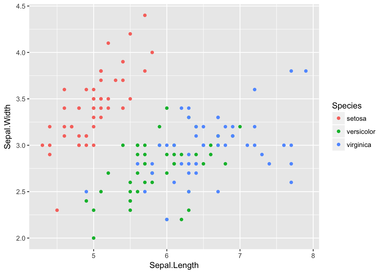
Or stuff for data exploration
## Warning: package 'psych' was built under R version 3.4.4##
## Attaching package: 'psych'## The following objects are masked from 'package:ggplot2':
##
## %+%, alpha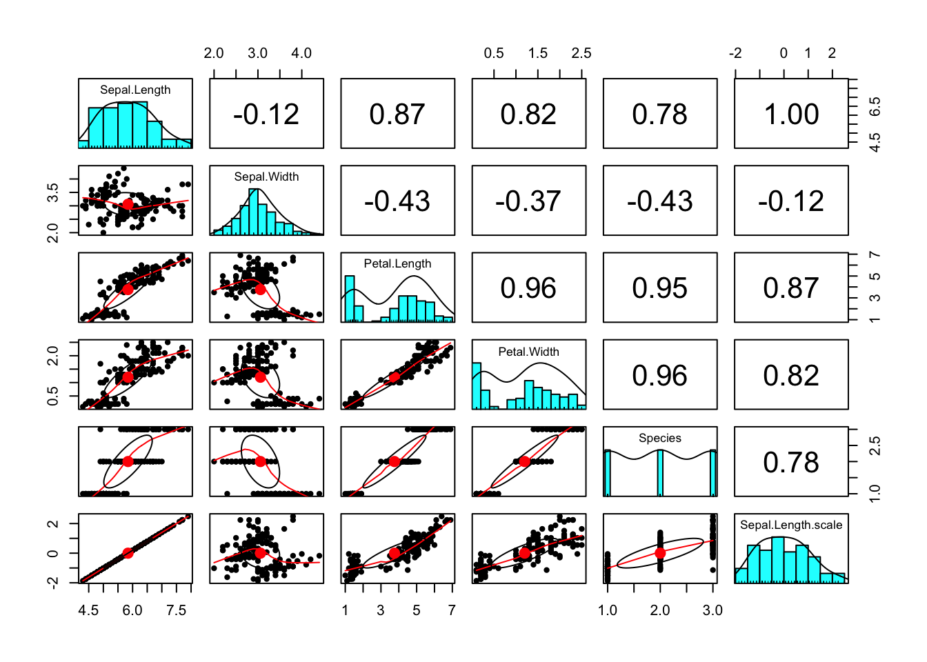
2.8 Functions for Psychologists
nlme()andlme4()for Multilevel Modelinglavaan()for Latent Variable AnalysisezAnova()for ANOVA based testing; the anova() function does model comparisons- profileR for Repeated Measures MANOVA
glm()andlm()for linear modelscaret()for Machine Learning
2.9 Resources
- swirl
- stackoverflow.com
- Your peers
- R Community
2.9.1 Template Stuff
You can label chapter and section titles using {#label} after them, e.g., we can reference Chapter 2. If you do not manually label them, there will be automatic labels anyway, e.g., Chapter ??.
Figures and tables with captions will be placed in figure and table environments, respectively.
Figure 2.1: Here is a nice figure!
Reference a figure by its code chunk label with the fig: prefix, e.g., see Figure 2.1. Similarly, you can reference tables generated from knitr::kable(), e.g., see Table 2.1.
| Sepal.Length | Sepal.Width | Petal.Length | Petal.Width | Species | Sepal.Length.scale |
|---|---|---|---|---|---|
| 5.1 | 3.5 | 1.4 | 0.2 | setosa | -0.89767388 |
| 4.9 | 3.0 | 1.4 | 0.2 | setosa | -1.13920048 |
| 4.7 | 3.2 | 1.3 | 0.2 | setosa | -1.38072709 |
| 4.6 | 3.1 | 1.5 | 0.2 | setosa | -1.50149039 |
| 5.0 | 3.6 | 1.4 | 0.2 | setosa | -1.01843718 |
| 5.4 | 3.9 | 1.7 | 0.4 | setosa | -0.53538397 |
| 4.6 | 3.4 | 1.4 | 0.3 | setosa | -1.50149039 |
| 5.0 | 3.4 | 1.5 | 0.2 | setosa | -1.01843718 |
| 4.4 | 2.9 | 1.4 | 0.2 | setosa | -1.74301699 |
| 4.9 | 3.1 | 1.5 | 0.1 | setosa | -1.13920048 |
| 5.4 | 3.7 | 1.5 | 0.2 | setosa | -0.53538397 |
| 4.8 | 3.4 | 1.6 | 0.2 | setosa | -1.25996379 |
| 4.8 | 3.0 | 1.4 | 0.1 | setosa | -1.25996379 |
| 4.3 | 3.0 | 1.1 | 0.1 | setosa | -1.86378030 |
| 5.8 | 4.0 | 1.2 | 0.2 | setosa | -0.05233076 |
| 5.7 | 4.4 | 1.5 | 0.4 | setosa | -0.17309407 |
| 5.4 | 3.9 | 1.3 | 0.4 | setosa | -0.53538397 |
| 5.1 | 3.5 | 1.4 | 0.3 | setosa | -0.89767388 |
| 5.7 | 3.8 | 1.7 | 0.3 | setosa | -0.17309407 |
| 5.1 | 3.8 | 1.5 | 0.3 | setosa | -0.89767388 |
You can write citations, too. For example, we are using the bookdown package (Xie 2017) in this sample book, which was built on top of R Markdown and knitr (Xie 2015).
References
Xie, Yihui. 2017. Bookdown: Authoring Books and Technical Documents with R Markdown. https://CRAN.R-project.org/package=bookdown.
Xie, Yihui. 2015. Dynamic Documents with R and Knitr. 2nd ed. Boca Raton, Florida: Chapman; Hall/CRC. http://yihui.name/knitr/.