Chapter 12 One Way ANOVA

In this chapter we are going to learn about the ANanalysis Of VAriance or the ANOVA. The ANOVA is a statistical technique that lets the analyst partition off where different sources of variation are coming from in controlled, experimental designs.

12.1 Theory

12.1.1 Type I Error Rates

If we are comparing more than two groups on their means, we should not use a t-test because performing multiple t tests across multiple groups in a single study increases the likelihood of at least one Type I error occurring across the “family” of comparisons. Experimentwise or familywise Type I error rate is equal to \[1 - (1-\alpha)^c\]

Where $c$ is the number of independent $t$ tests to be conducted.

For example, if I wanted to conduct a test for each pairwise comparison in a 3-group study, my experiment-wise error rate would be \[1 –(1 -.05)^3= .142.\] The three comparisions would be between

Group 1 and Group 2
Group 1 and Group 3
Group 2 and Group 3.

For 4 conditions, it would be 6 tests. Those six tests would be between

Group 1 and Group 2
Group 1 and Group 3
Group 1 and Group 4
Group 2 and Group 3
Group 2 and Group 4
Group 3 and Group 4

And the formula would look like this:

\[1 –(1 -.05)^6= .265\]

We can find the number of comparision that we are going to do with the formula $\frac{k(k-1)}{2}$.

12.1.2 The F Test

The ANOVA or F test controls Type I error rrate while simultaneiously allwoing a test of the equality of multiple population means. The one-way ANOVA is used to analyze data generated by the manipulation of one independent variable with at least 2 levels. Each group, or condition, created by the manipulation is called a level. The null hypothesis for an ANOVA is \[H_0 : \mu_1 = \mu_2 = ... = \mu_k\] The alternative hypothesis is: \[H_a: \mu_i \neq \mu_k\]

The idea behind the ANOVA is that we use two estimates of the population variance associated with the null hypothesis.

One estimate is the within-group variation or $s_W^2$ which is the influcen on variance due to error which is presumed to be the same in each group $\sigma_e^2$.
The other is the actual effect we are trying to islate. This is the between-group variation or $s_B^2$: the influence on variance due to the independent variable or treatment $\sigma_t^2$, plus the error due to the random process of group asigmment or $\sigma_e^2$.
The test statistic involves creating a ratio of the between-groups to within group variation.

With the ANOVA we have variance calculated on both the top and bottom.

\[\frac{\sigma_e^2+\sigma_t^2}{\sigma_e^2}=\frac{s_B^2}{s_W^2}\]

12.1.3 The Grand Mean

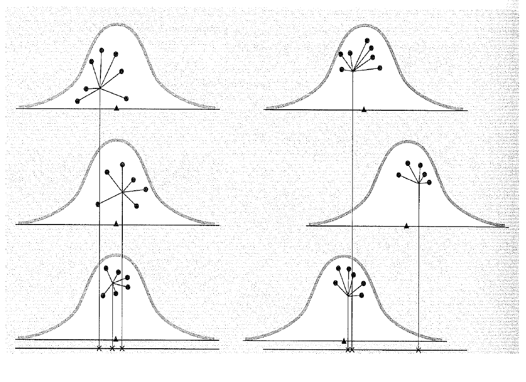
Every given score in a data set differs somewhat from the overall, or grand, mean of the data set. But this distance from the grand mean can be partitioned into the distance from the score to its group mean and the distance from that group mean to the grand mean.

[Image of multiple population means]

An individual score in an ANOVA model comprises of 3 components. The linear model is $X_{ik}=\mu+\alpha_k+e_{ik}$. In this equation $\mu$ is the grand mean, $a_k$ is the effect of belonging to the respective group $k$. And then $e_{ik}$ is random error.

The distance from a score to its group mean essentially reflects error only, whereas the distance from a group mean to the grand mean reflects the effect of the treatment + error.

Knowing that we are looking at total variation in the data set, we can then split all the variation into within groups variation (noise) and between groups variation(signal). In terms of the toal variation, or the sums of squares, we can represent this as \[SS_T = SS_W + SS_B\]

[EXAMPLES HERE OF CHANGING SS BETWEEN AND WTIHIN GROUPS]

[WHY WE CALL IT SUMS OF SQUARES, REFER BACK TO T TEST]

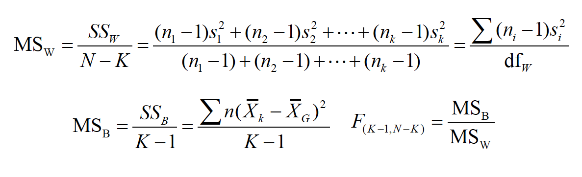
These SS or Sums of Squares must then be divided by their respective df to obtain the estiamtes of the average variability within groups and the average variability between groups. We can calculate each part of the total sums of squares below. First, the mean square within:

\[MS_W = \frac{SS_W}{N-K} = \frac{(n_1-1)s_1^2 +(n_2-1)s_2^2 + ... + (n_k-1)s_k^2}{(n_1 -1)+(n_2 -1)+...+(n_k-1)}=\frac{\Sigma(n_i-1)s_i^2}{df_w}\]

Walking through this equation, we see that we are trying to calculate the within subjects sum of squares. Remember this is the amount of noise associated with each group. If this number is very small, it means that whatever our experiment was is going to be very good at capturing the effects. On the top of the equation, we calculate the within group sum of squares. We subtract 1 from each observation, the multiply that by the group’s variation and then add them all up. This notation is simplified with the $\Sigma$ notation. The denominator is then just the total amount of individual observations or $N$, subtract the number of groups, $K$.

We calculate the mean square between with the equation below

\[MS_B = \frac{SS_B}{K-1}=\frac{\Sigma n(\bar{X_k}-\bar{X_G})^2}{K-1}\]

Here we are going just like above add up the mean from every group’s mean subtract the grand mean, while multiplying that number by the amount of observations that went into that group [not clear]. We then divide that summation by $K-1$.

Finally we then divide the between group sum of squares by the within group sum of squares. We use $K-1,N-K$ as our degrees of freedom. Note that we now have 2 values for our degrees of freedom!

\[F_{(K-1,N-K)}=\frac{MS_B}{MS_W}\]

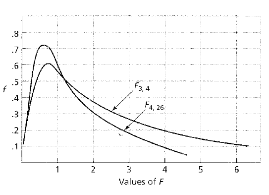
If there is no treatment effect due to the independent variable (i.e., the null hypothesis is true), then we expect this ratio to be roughly equal to 1.

12.1.4 ANOVA Assumptions

To be representative of the populations from which they were drawn, the observations in our samples must be random and independent.
The population distributions from which our samples were drawn are normal, which implies that our dependent variable is normally distributed.
The variances of our population distributions are equal (homogeneity of variance).
Generally speaking, the ANOVA is robust to minor violations of the normality and variance assumptions, except for cases in which heterogeneity is coupled with unequal sample sizes

12.2 Practice

Let’s try this out! Imagine the following reserach question:

Scenario: Does the ethnicity of a defendant affect the likelihood that he is judged guilty? People were given transcripts of a trial and asked to judge the likelihood that a defendant was guilty, on a 0 –10 scale. The transcript was identical, but across 3 conditions, the reported ethnicity of the defendant varied. The results were as follows (study based on Stephen, 1975):

12.2.0.1 Step One

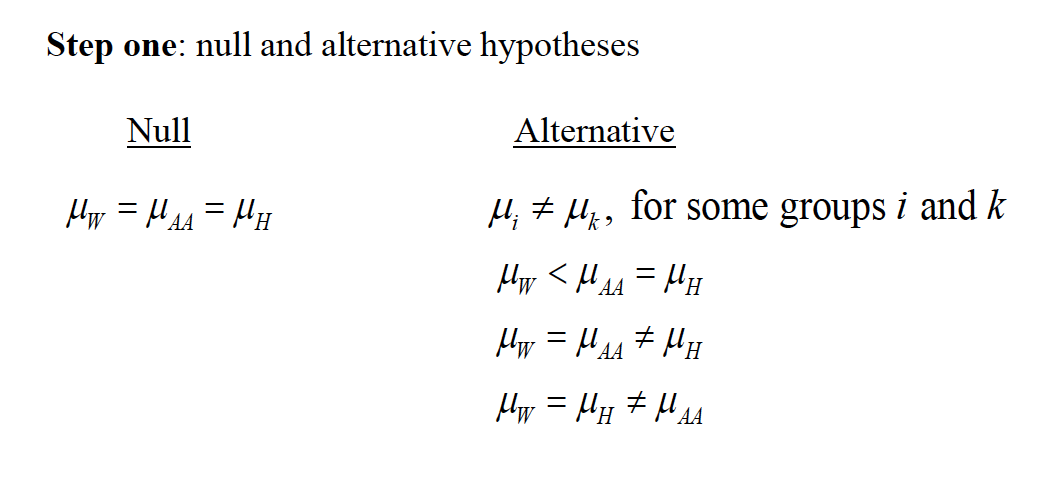
The first step in the process is to state the null and alternative hypothesis.

$H_0: _W = _B = _H $ $H_A: _i u_k $ For some groups i and k. Note that the hypothesis is only that all the groups just don’t have the same mean. Nothing is said yet about what groups will be higher or lower!!

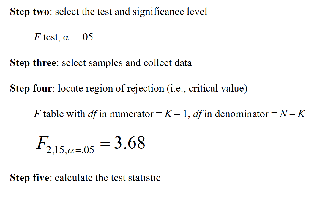
12.2.0.2 Step Two

Select the test and significance level. In this case we are going to use an $F$ test with an $\alpha = .05$.

12.2.1 Step Three

Let’s enter in the data:

# SHOULD BE DIFFERENT FORMAT GOING IN TO SAVE HEADACHE
white <- c(6,7,2,3,5,0)
black <- c(10,9,4,10,10,3)
hispanic <- c(10,6,5,5,2,10)
defendantData <- data.frame(white,black,hispanic)

12.2.1.1 Step Four

Locate the region of rejection aka the critical value. We know that we have 18 total observations and three groups. Knowing the formula is $F_{(K-1,N-K)}$ we calculate our $df$ to be $F_{(3-1,18-3)}$ or $F_{(2,15)}$ which on our F distribution table comes out to be 3.68.

12.2.1.2 Step Five

Calculate the test statistic!

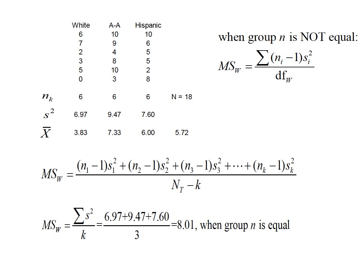
Using the formuala from above, we first figure the variance and the means associated with each group.

\[MS_W = \frac{SS_W}{N-K} = \frac{(n_1-1)s_1^2 +(n_2-1)s_2^2 + ... + (n_k-1)s_k^2}{N_T - k}\]

\[MS_W = \frac{\Sigma s^2}{k} = \frac{6.97 +9.47 + 7.60}{3}=8.01\]

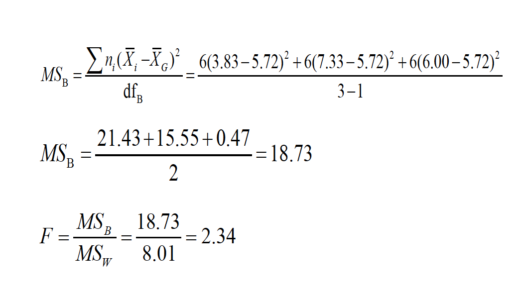
Then for the mean square between.

\[MS_B=\frac{\Sigma n(\bar{X_k}-\bar{X_G})^2}{K-1}=\frac{6(3.83-5.72)^2+6(7.33-5.75)^2+6(.00-5.72)^2}{3-1}\]

Which reduces to

\[MS_B=\frac{21.43+15.55+0.47}{2}=18.73\]

And then we use both of these values to see if the two values when divided exceede our test statistic.

\[F=\frac{MS_B}{MS_W}=\frac{18.73}{8.01}=2.34\]

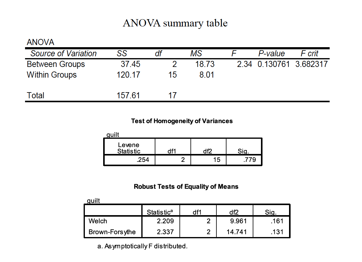
12.2.1.3 Step Six

We then interpret.

We do NOT reject the null, because the $F$ value did not exceed the $F_{cv}$. And we would write it up by saying:

“The ethnicity of the defendant did not significantly affect the average guilt rating given by mock jurors, F(2, 15) = 2.34, p> .05.”

[DB LEFT HERE]

12.2.2 Running The Calulation in R

Let’s run the same data in R to see what happens! The first thing we need to do is melt our data so it’s in a long, not wide format.

# ENTER HERE

In cases where the number of groups in a study (K) is more than two, we cannot use the ttest for the hypothesis test because there is an associated cost. 2. The Analysis of Variance (ANOVA), or Ftest, controls the experimentwiseType I error rate while simultaneously allowing a test of the equality of multiple population means. 3. Every given score in a data set differs somewhat from the overall, or grand, mean of the data set. But this distance from the grand mean can be partitioned into the distance from the score to its group mean and the distance from that group mean to the grand mean. 4. There are several assumptions that should be met when using ANOVA. 5. The steps of the hypothesis test for ANOVA 6. Effect size and power for the ANOVA

Performing multiple ttests across multiple groups in a single study b. Experimentwise(familywise) Type I errorrate = 1 –(1 –α)c, where c= number of independent ttests to be conducted

The one-way ANOVAis used to analyze data generated by the manipulation of one independent variable with at least 2 levels. Each group, or condition, created by the manipulation is called a level. b. The null hypothesis—H0: c.The alternative hypothesis—Ha: , for some pair of groups iand k

The concept behind the ANOVA is that we use two estimates of the population variance associated with the null hypothesis i. One estimate is the within-groups variation ( ): the influence on variance due to error (chance factors like individual differences), which is presumed to be the same within each group ( ) ii. The other estimate is the between-groupsvariation ( ): the influence on variance due to the independent variable or treatment ( ), plus error due to the random process of group assignment ( )

The test statistic involves created a ratio of the between-groups to the within-group variation:

Obtaining estimates of variance in our data is the trick in the ANOVA. a. An individual score in an ANOVA model is comprised of 3 components. The linear model is , where μis the grand mean, αkis the effect of belonging to group k, and eikis random error. b. The distance from a score to its group mean essentially reflects error only, whereas the distance from a group mean to the grand mean reflects the effect of the treatment + error

Obtaining estimates of variance in our data is the trick in the ANOVA. c. The total variation in a data set, then, can be split into that due to within-group variation + between-group variation. In terms of sums of squares: d. These SS estimates must be divided by their respective dfto obtain the estimates of the average variability within-groups and the average variability between-groups.

three

F STATISTIC FROMULA

If there is no treatment effect due to the independent variable (i.e., the null hypothesis is true), then we expect this ratio to be roughly equal to 1.

However, if there is a treatment effect due to the independent variable (i.e., the null hypothesis is false), then we expect this ratio to be > 1.

three

12.2.3 Assumptions of ANOVA

To be representative of the populations from which they were drawn, the observations in our samples must be random and independent.
The population distributions from which our samples were drawn are normal, which implies that our dependent variable is normally distributed. c.The variances of our population distributions are equal (homogeneity of variance). d.Generally speaking, the ANOVA is robust to minor violations of the normality and variance assumptions, except for cases in which heterogeneity is coupled with unequal sample sizes

12.2.4 Practice

white <- c(6,7,3,2,3,5,0)
black <- c(10,9,4,10,10,3)
hispanic <- c(6,10,5,5,10,2)

three

anova

Step six: Interpret (was null rejected?). We do NOT reject the null, because the Fvalue did not exceed the Fcv “The ethnicity of the defendant did not significantly affect the average guilt rating given by mock jurors, F(2, 15) = 2.34, p> .05.”

12.3 Effect Size Measures

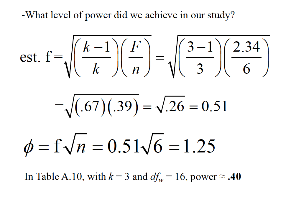
An effect size measure, f, is used to represent the population SD between groups from the grand mean, versus population SD within a group

anova

We can then use the noncentrality parameter for the Fdistribution, related highly to phi, to estimate power

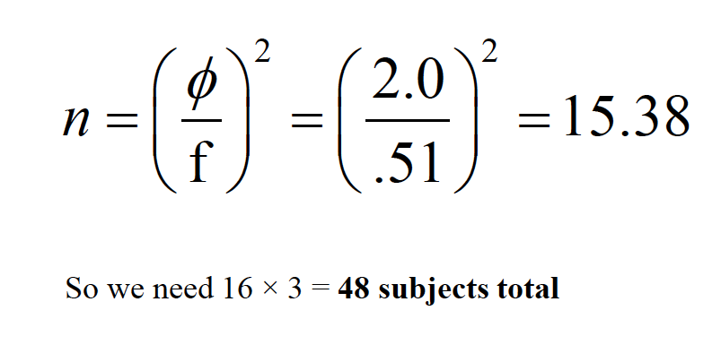
$\phi = f * \sqrt{n}$ $n = \frac\{\phi}{f}^2$

Consult Table A.10 for values of phi, based on number of groups (K) and the likely dfw(although this has a modest influence)

$n = \frac\{\phi}{f}^2$

What if we desired .80 power? How many subjects?

In Table A.10, with k= 3 and dfw= 16, phi = 2.0

anova

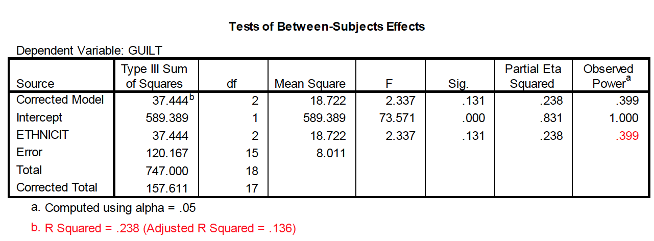
This type of measure is comparable to R2in regression Interpretation: roughly 28% of the variance in the DV (i.e., guilt ratings) can be attributed to the IV (i.e., the race of the defendant). But it is upwardly biased—it overpredictsthe population eta-squared

anova

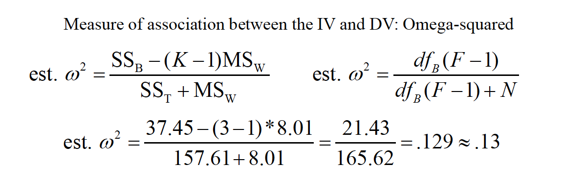
Interpretation: roughly 13% of the variance in the DV (i.e., guilt ratings) can be attributed to the IV (i.e., the race of the defendant).

Cohen (1977) recommends the following convention: ≈ .01 is “small” ≈ .06 is “medium” ≥.15 is “large”

Look for “adjusted R squared” notation in the SPSS ANOVA output from the Univariatemethod of performing the ANOVA

anova