Chapter 13 Multiple Comparisons
In past lectures we have discussed the problem with the familywise (or what your text calls “experimentwise”) Type I error rate.
There are different methods for holding the familywise error rate at no more than .05. This methodology is most commonly used in post hoc tests designed to test specific contrasts among conditions following a significant ANOVA.
In addition to comparisons done post hoc, others can be done a priori, commonly known as planned comparisons. Because such comparisons are usually done with a particular theoretical outcome in mind, they are not as conservative as post hoc comparisons.
- Familywise Type I error rate = , where j = number of independent t tests to be conducted.
- When comparisons are not independent, the familywise rate can be approximated by the formula .
- The comparisonwise error rate is the Type I error rate per comparison.
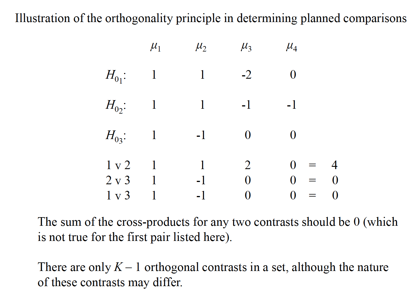
- Comparisons are orthogonal if the outcome of one test is not redundant with the outcome of another. There are (k – 1) orthogonal comparisons in a data set, which will be discussed in more detail.
There are different methods for holding the familywise error rate at no more than .05. This methodology is most commonly used in post hoc tests designed to test specific contrasts among conditions following a significant ANOVA.
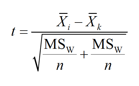
The simplest, and most powerful test, is called the Fisher Least Significant Difference test (LSD). It is sometimes called the “protected t” test, and the formula is:
IMG
You then use the df from the overall error term for finding the critical value of t. This test should be used only following a significant F test, and for no more than 3 groups. If homogeneity of variance is not tenable, then use the individual variances from the groups being tested, as the case for a traditional separate variances t test with df = N - 2.
How does the Fisher LSD protect against Type I error inflation with only 3 groups?
Complete null is true
\(H_0 : \mu_1 = \mu_2 = \mu_3\)
In this case, if the overall F is significant, you have already committed a Type I error and any more of them don’t contribute further to αFW (i.e., you are just going to commit the ‘same’ error in a particular pairwise comparison. This is the case no matter how many groups are in the experiment.
Partial null is true
\(H_0 : \mu_1 = \mu_2 != \mu_3\)
With 3 groups, if the overall F is significant, it was not a Type I error; there is only one real chance of a Type I error—that being when the partial null is true. Here αFW was never in danger of being more than .05. But with more than 3 groups, and when more than one partial null is true, you have the chance of committing multiple errors.
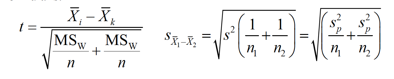
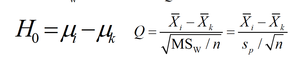
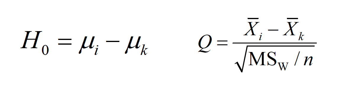
Another common method is to use the studentized range (Q) sampling distribution as the source of critical values for minimum differences needed to declare population means significantly different.
The Tukey method computes the minimum difference needed for any pair of means to be significantly different. We use alpha, the number of means being compared (r), and the df associated with MSW to find a critical Q value.
Image
With this method, you are protecting yourself against the most extreme possible Type I error (i.e., between the largest and smallest means), and therefore all other comparisons are likewise protected.
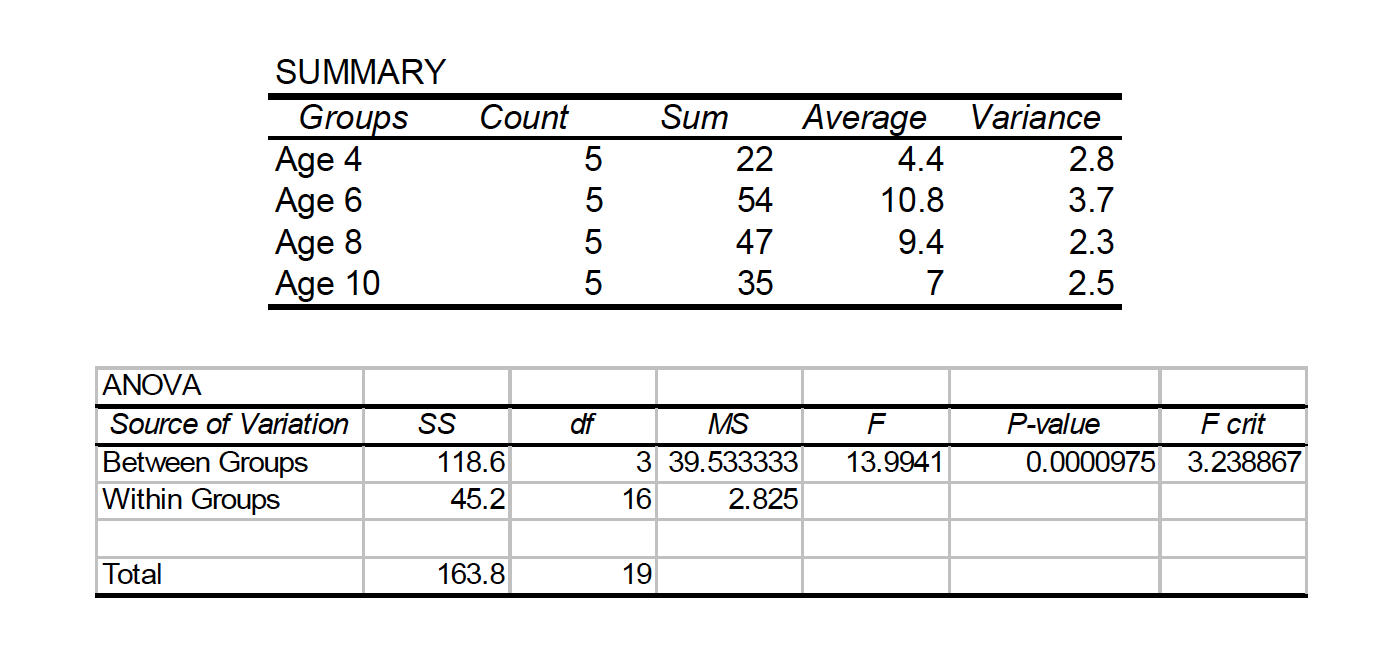
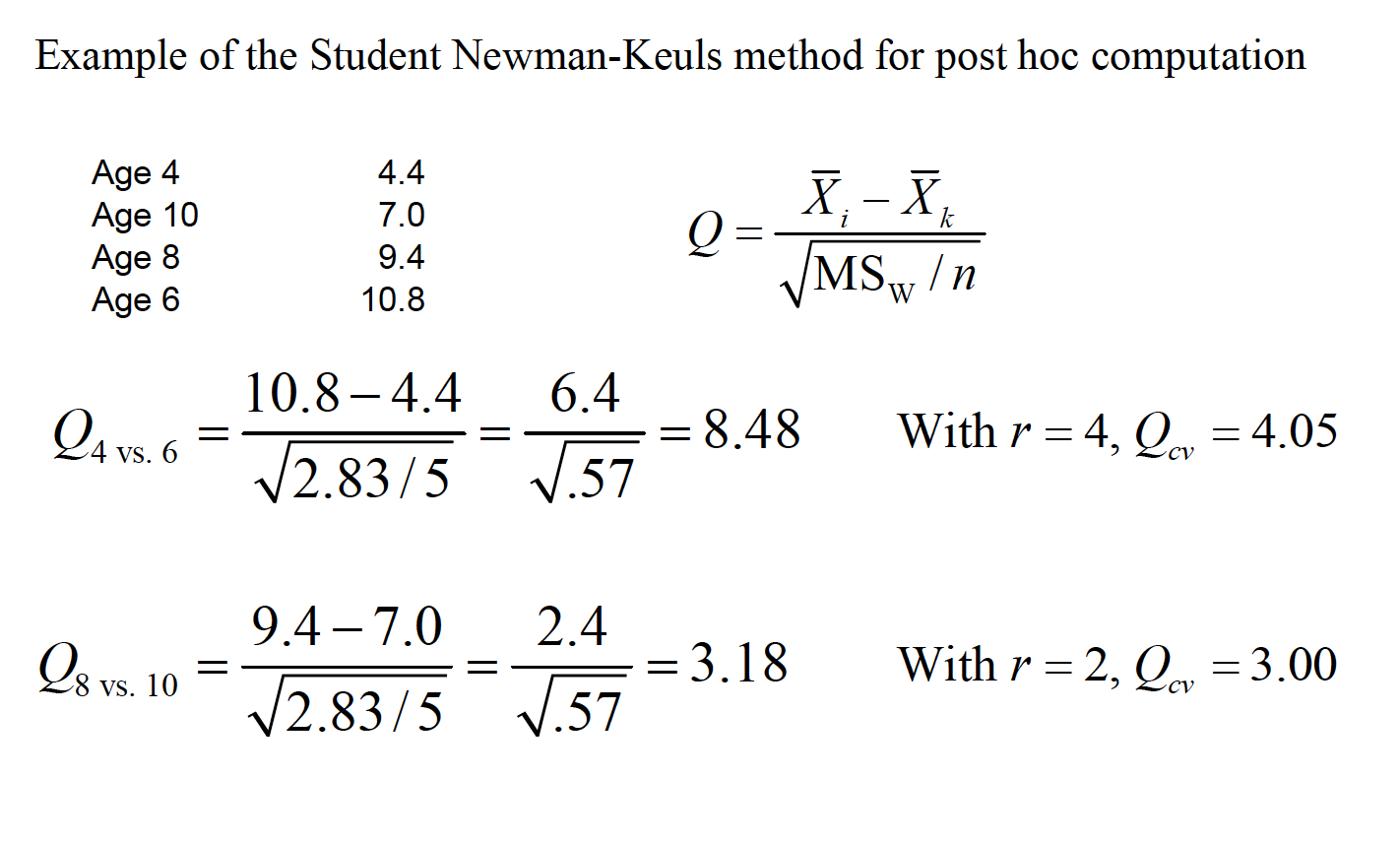
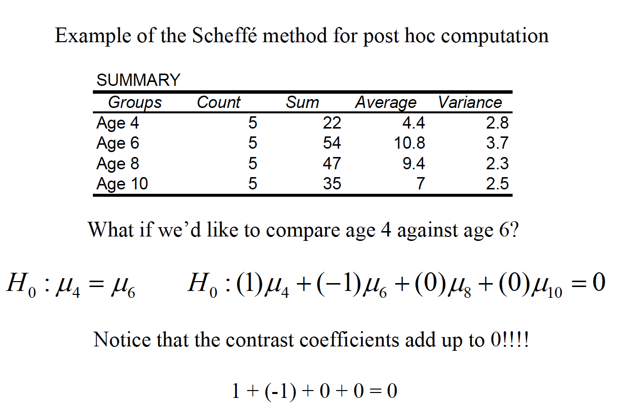
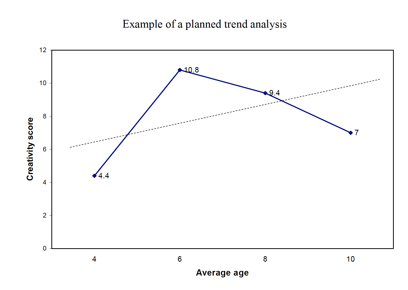
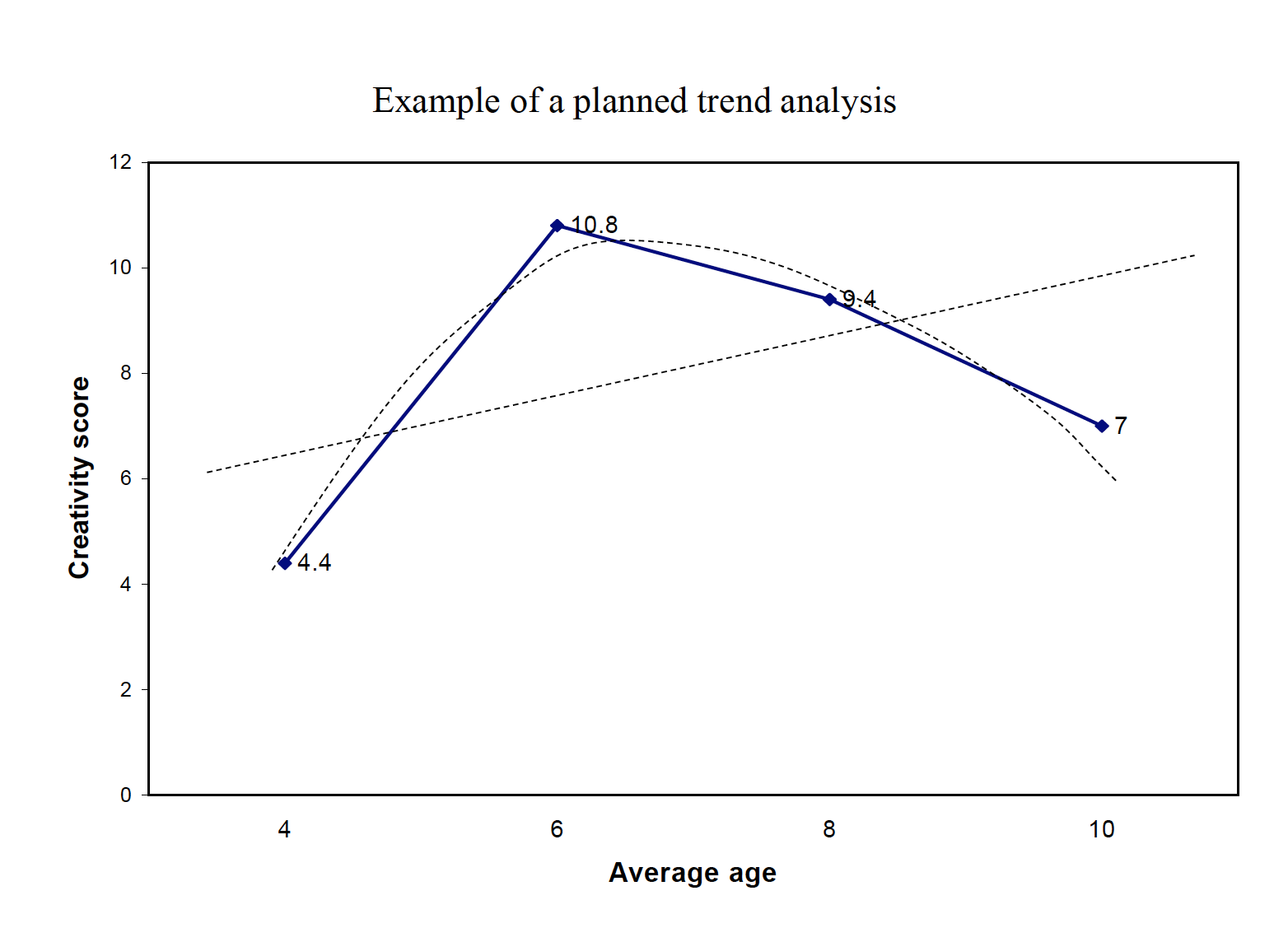
Scenario: A researcher gives a test of creativity to four groups of children. The age difference between each group is 2 years (range 4-10 years). Do the children demonstrate significantly different levels of creativity?
Image
Image
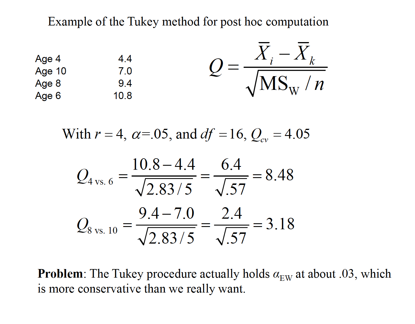
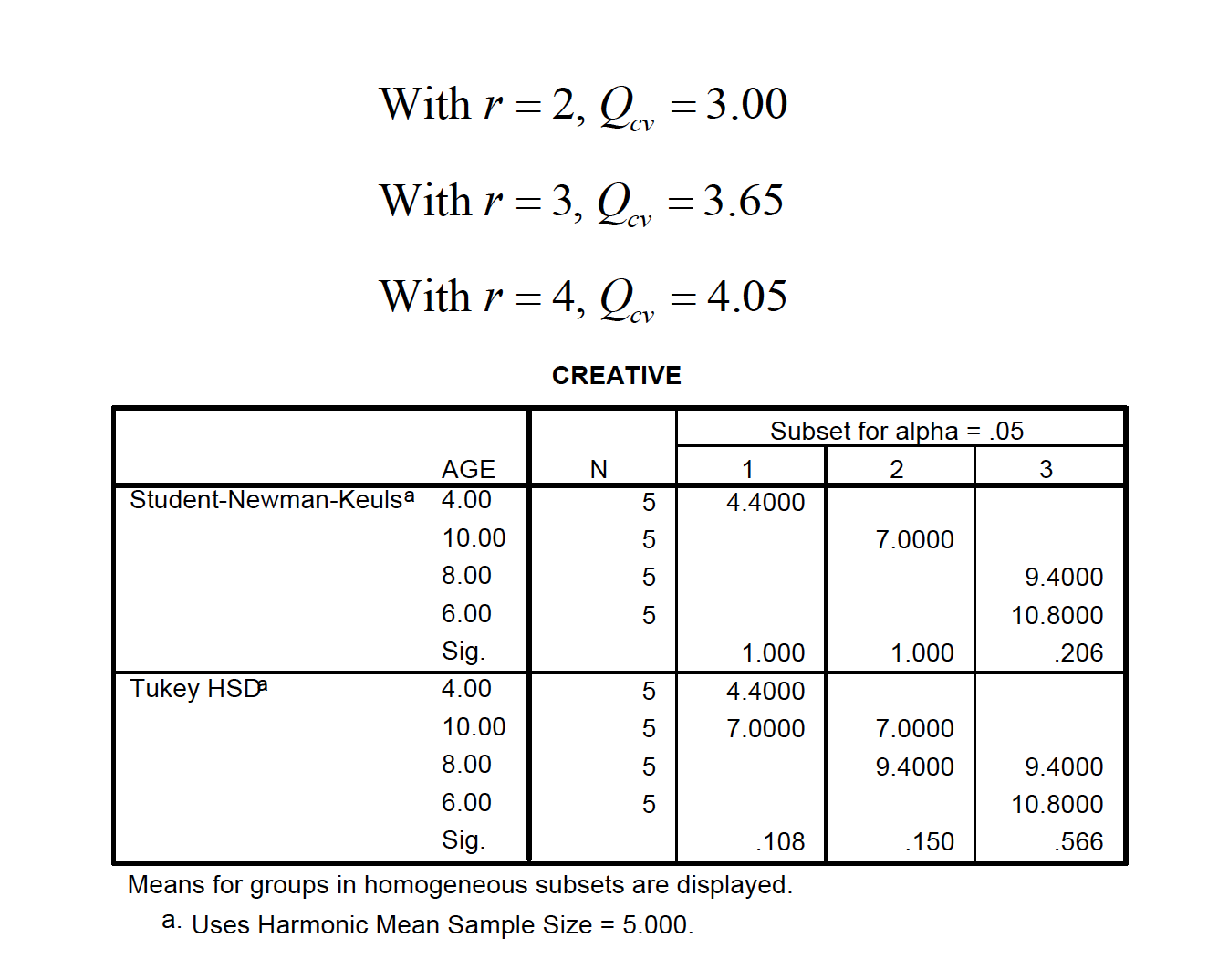
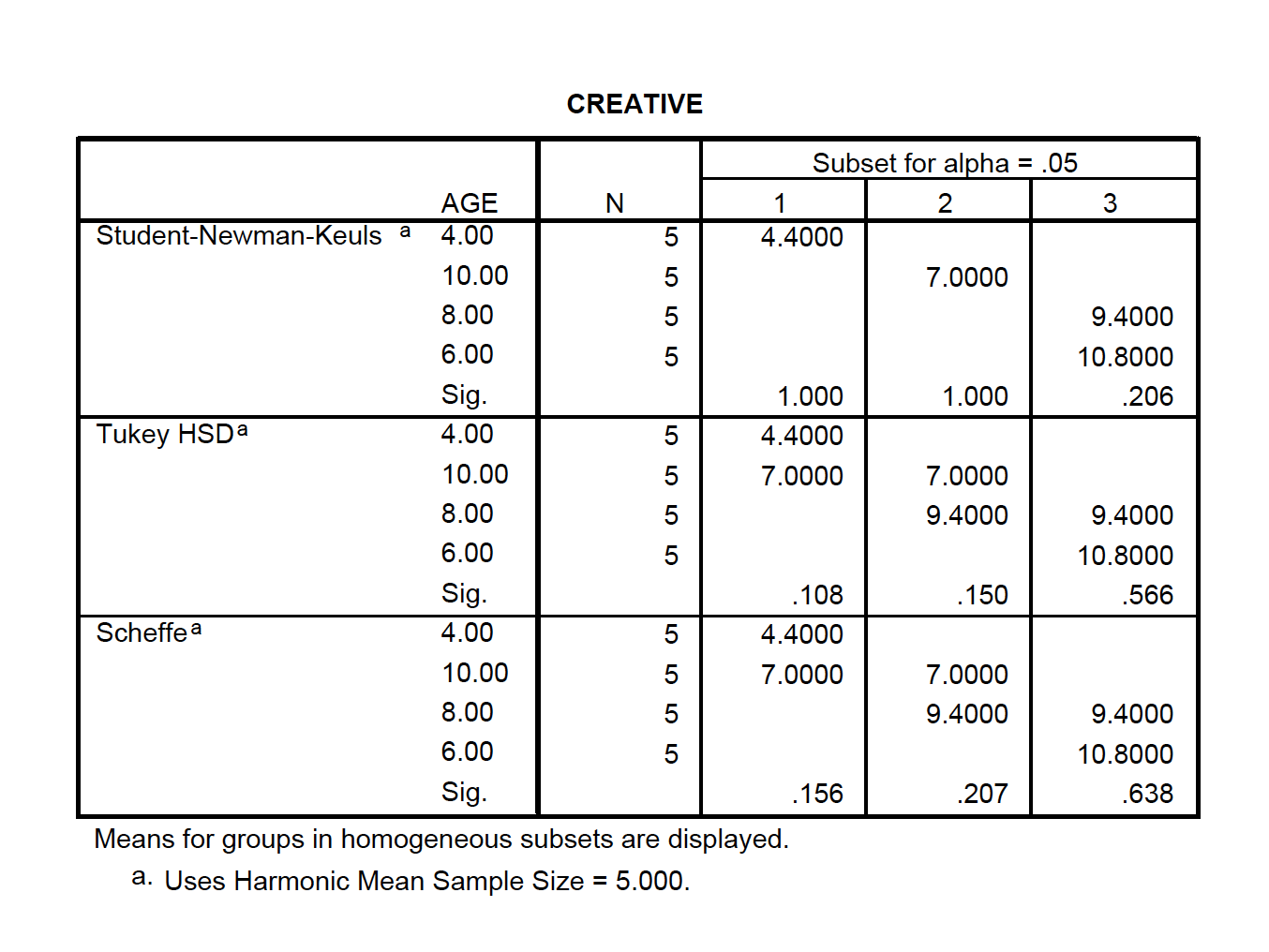
The Student Newman-Keuls method is similar to the Tukey, except that the critical value is determined by the number of steps separating each pair of means (r): range = i – k + 1
Problem: we do lose some control over αEW, as it actually goes over .05
Image
Image
Image
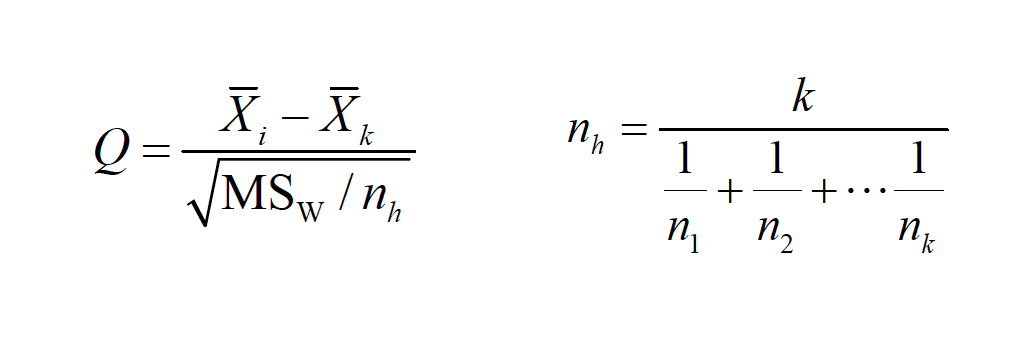
The Tukey/Kramer method is used when sample sizes are unequal. We calculate the harmonic mean of the sample sizes to achieve the appropriate number in the denominator:
Image
The Ryan (or REGWQ) test is a modification of the SNK to achieve increased power but also keeps αEW no greater than .05. It is preferred over Tukey to get better power and over SNK to keep αEW ≤ .05. This means it uses fractional values of alpha that are not easy to tabulate—but SPSS and other packages offer it as an option so it’s easy to use.

Image
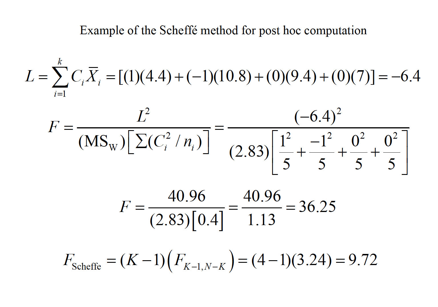
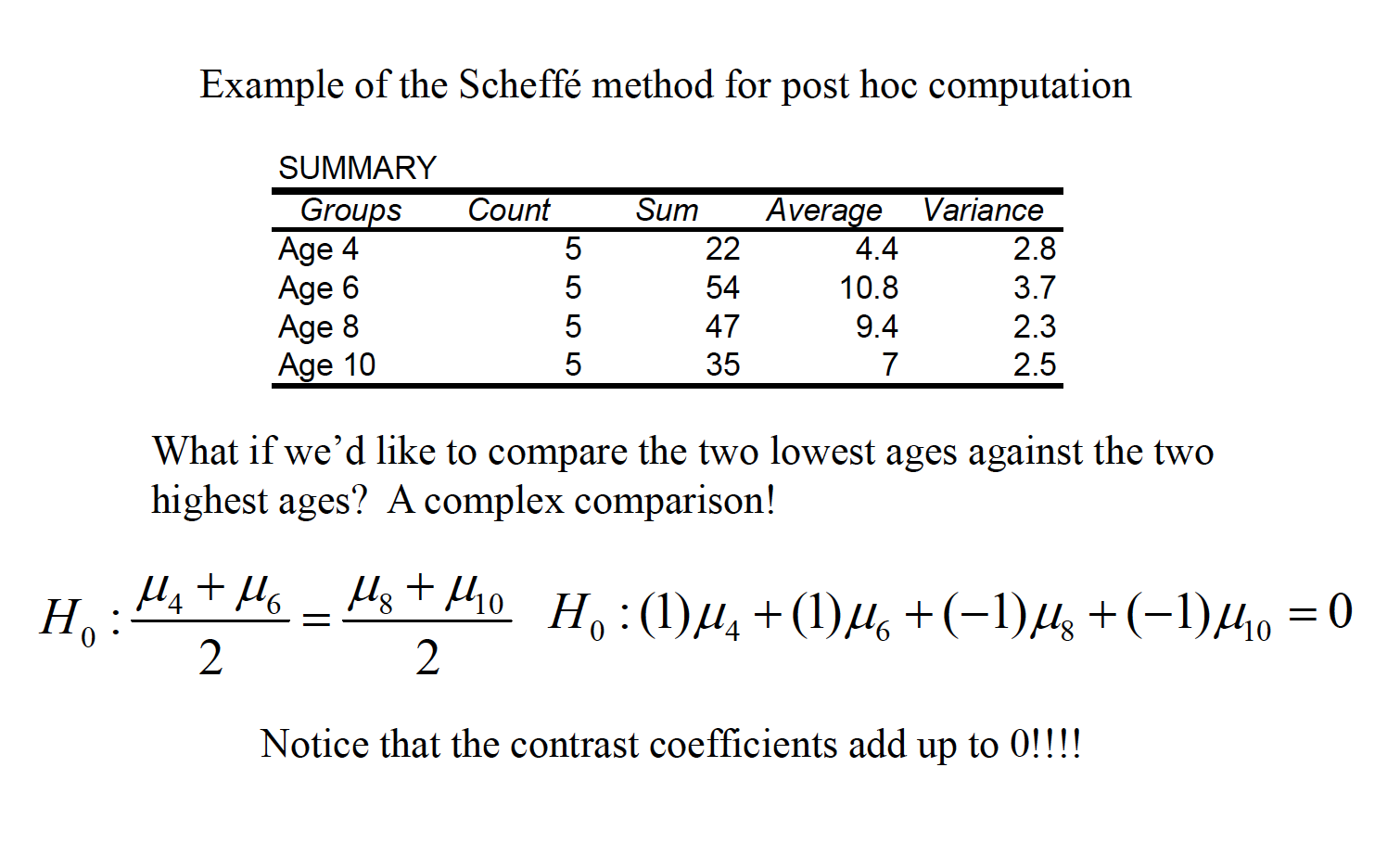
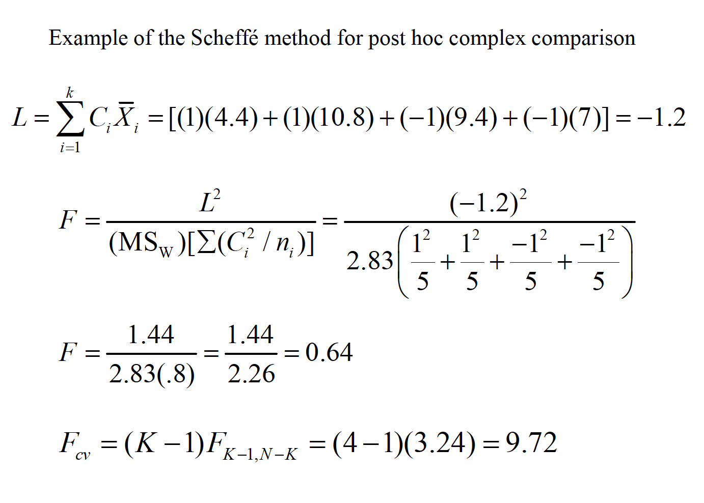
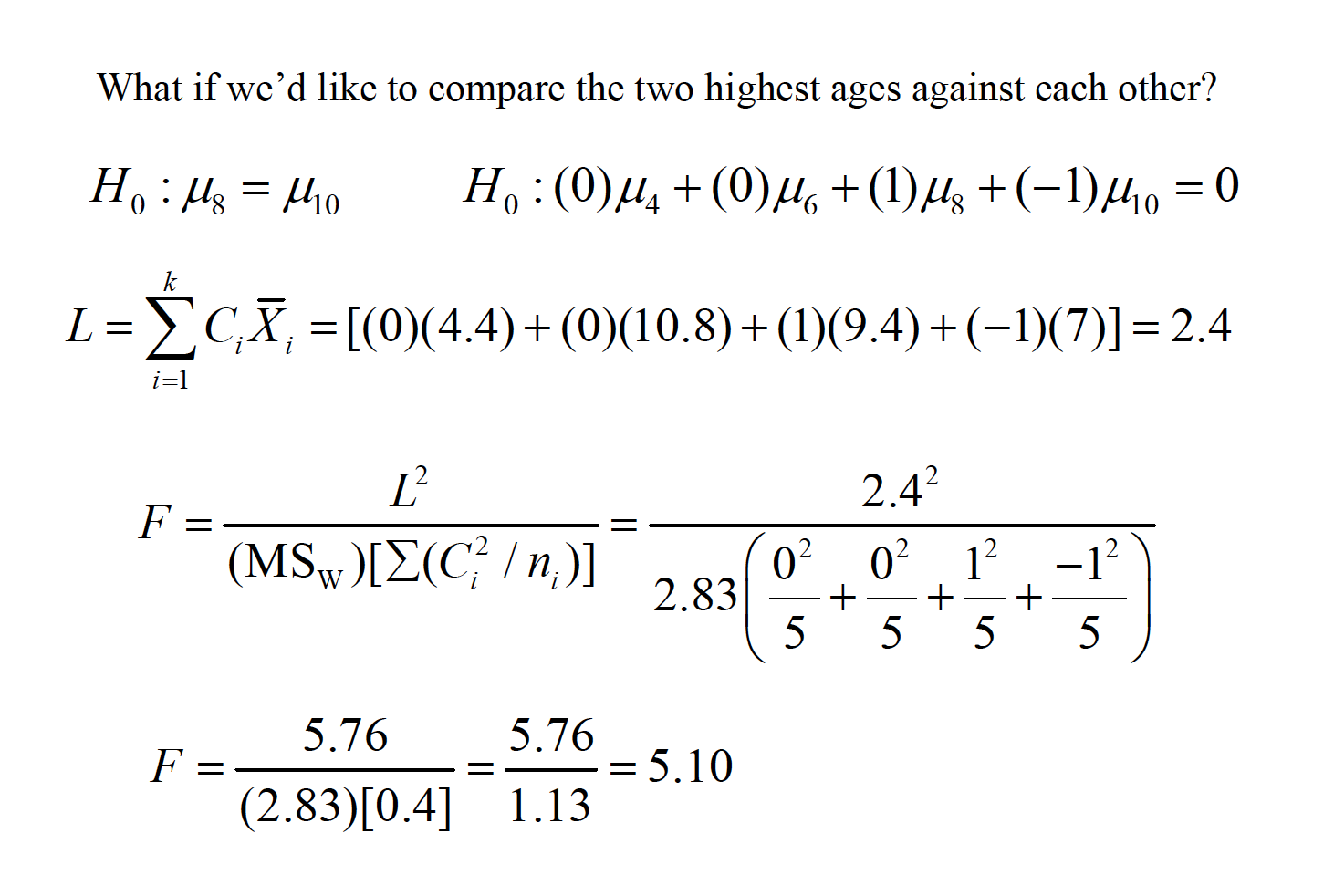
Another conservative method, the Scheffeaccent test, uses the F distribution, but can also be used to test complex comparisons involving combined groups, called linear contrasts.
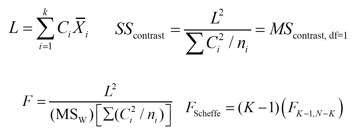
Image
The critical value of F sets the experimentwise error rate against all possible linear contrasts, not just pairwise contrasts.
Image
Image
Image
Image
Image
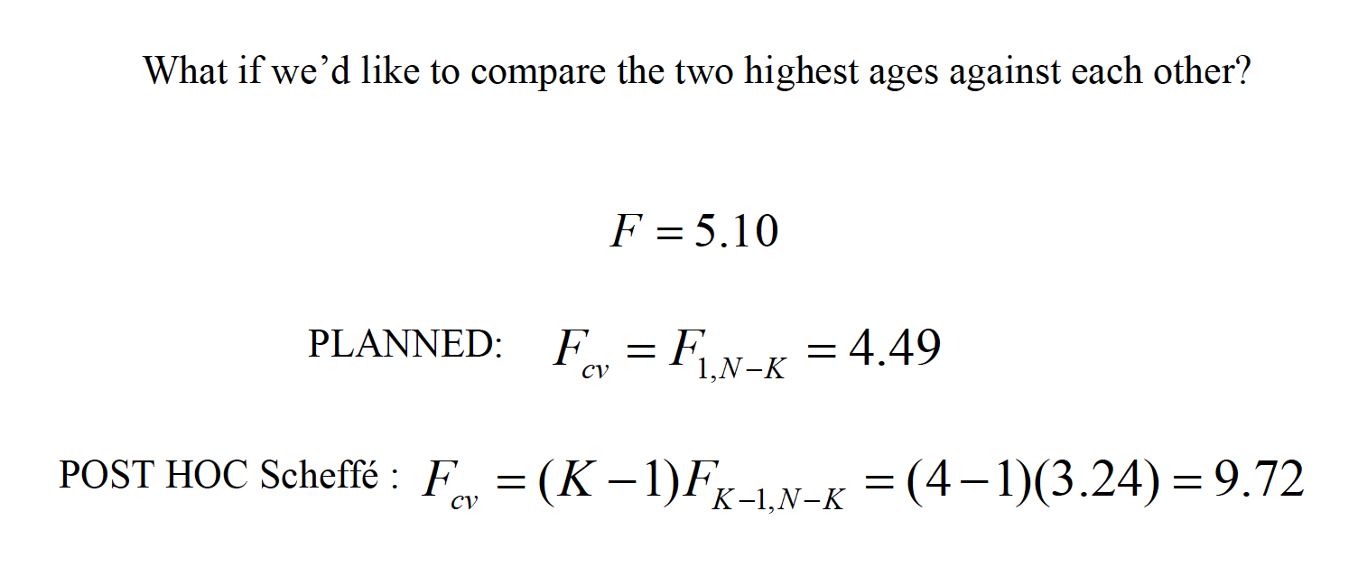
In addition to comparisons done post hoc, others can be done a priori, commonly known as planned comparisons. Because such comparisons are usually done with a particular theoretical outcome in mind, they are typically not as conservative as post hoc comparisons.
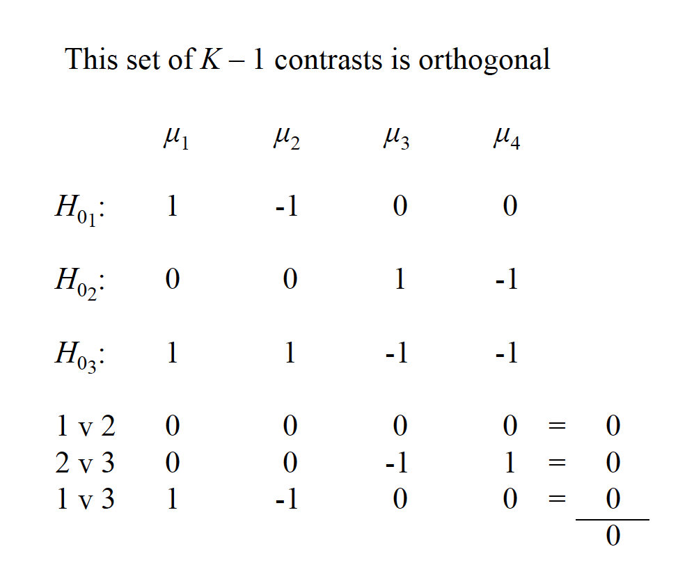
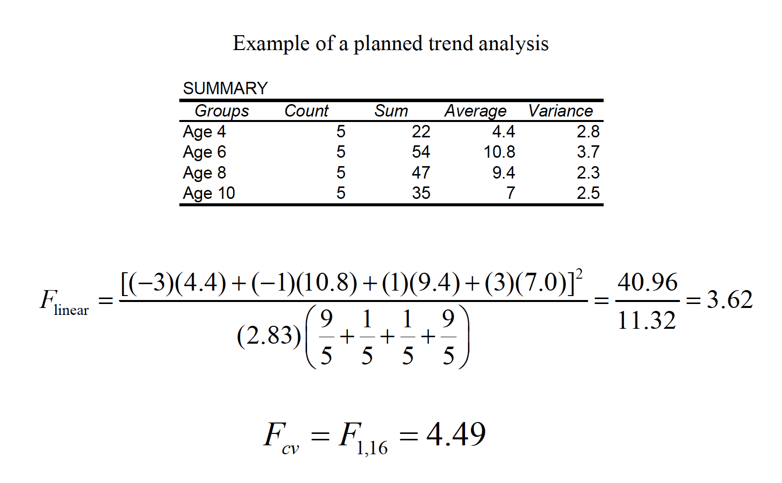
The linear contrast described earlier is generally used to complete planned comparisons. There are two primary differences as compared to the post hoc version of the test. If multiple contrasts are to be done, then it’s best if they are orthogonal, or independent. There are K – 1 orthogonal comparisons available in any one set of contrasts. Most (e.g., your text author) argue that you can keep each contrast at α = .05 when the set is orthogonal.
The linear contrast method described earlier is also used to complete planned comparisons. There are two primary differences as compared to the post hoc Scheffé test. Because of the orthogonality principle, the critical value for each comparison allows for more power (i.e., it is more liberal than the post hoc version Scheffé developed):
\(F_{cv}=F_{1,N-K}\)
Image
Image
A very conservative, but simple, method is to figure the comparisonwise error rate is to divide the familywise error rate by the number of comparisons one wishes to make. This is known as the Bonferroni test or the Dunn test.
\(\alpha_{pc}= \alpha_{EW}/J\)
For example, with 3 comparisons, α = .05/3 = .0167. You don’t set the modified alpha based on all possible comparisons, just based on the number you wish to conduct.
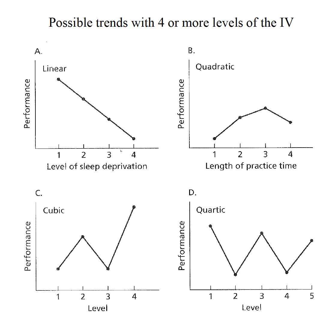
13.1 Trend analysis
A statistical procedure called trend analysis can be done to examine the functional relationship between a quantitative IV and the DV (e.g., linear, quadratic, cubic).
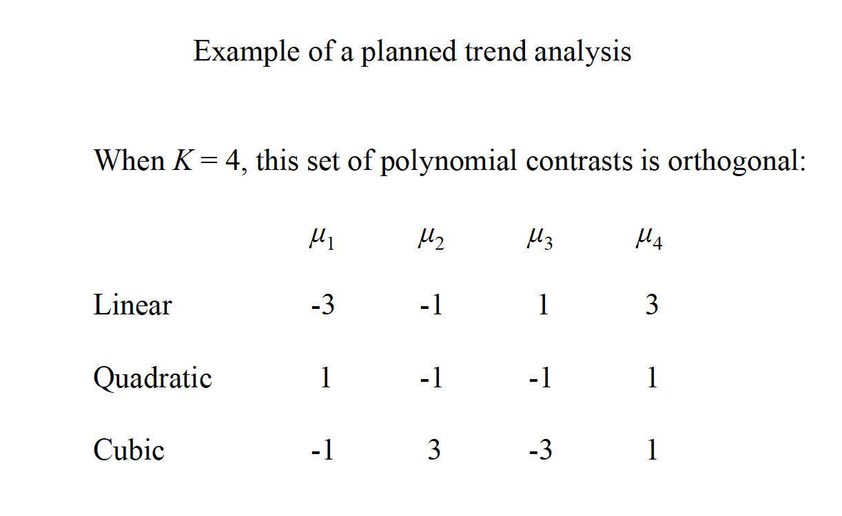
The same linear contrast comparison method is used as with regular contrasts, and the trend contrast coefficients are a special set of orthogonal comparisons based on K.
Image
Image
Image
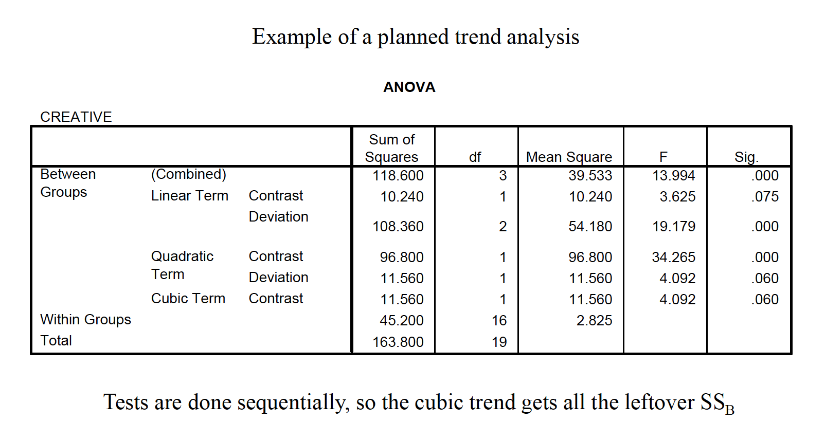
A statistical procedure called trend analysis can be done to examine the functional relationship between a quantitative IV and the DV (e.g., linear, quadratic, cubic). Trend analysis works only when the IV is a quantitative variable (e.g., drug dosage). More than one trend may be significant, and therefore inspecting a graph of the means in tandem with the analysis is highly recommended.
Image