Chapter 24 ANCOVA
24.1 Theory
24.1.1 Reducing Noise
Just like the ANOVA (Analysis of Variance), the ANCOVA (Analysis of Covariance) is used to analyze experiments by calculating an F ratio for more than 2 groups. As with any F calculation, differences in the dependent variable are caused by two things:
- The independent variable (signal, systematic variation)
- Error (noise, unsysematic variation)
The F statistic captures this
\[ F = \frac{Variation\ Due\ to\ IV}{Variation\ Due\ to\ Error} \]
When there is small variation within groups and large variation between groups, we get a large F.
CHART HERE
When there is large variatin within groups and small variation between groups, we get a small F.
The idea with the ANCOVA is that you can reduce your error term (the denominator from above) by choosing a covariate (CV) that is related to the DV and will soak up some random variation in your F test to give you a clearer picture of what is going on. Usually this means controlling for some sort of variable. The classic example is if you wanted to give some kids a test of some mental ability in a between subjects design but you don’t want their age to skew your results. You might have had a control condition, an intervention, and some sort of alternate intervention. Typically you would run an ANOVA on the three groups, but since you know age has been accounted for and you want to remove that effect from the model, you enter age as a covariate in this calculation. Outside of this there are three major applications for ANCOVA.
- Increase test sensitivity by using the CV(s) to account for more of the error variance
- Adjust DV scores to what they would be if everyone scored the same on the CV(s)
- Adjustment of a DV for other DVs taken as CVs
Note that use of a CV can adjust DV scores and show a larger effect or the CV can even eliminate the effect. Looking at this another way:
- Reduces random error by increasing the size of F
- Reduces systematic error by adjusting for differences in means
- May increase differences by soaking up error
It’s a good idea to use ANCOVA when you are removing variance in the DV related to covariate, but not related to the grouping variable. This decreases the error term and increases power.
It’sa bad idea to use ANCOVA when groups differ on their mean level of the covariate. Usually here the covariate and the grouping variable are not independent. An example of this might be when “controlling” for anxiety when studying people with and without depression. Clearly people with depression will have higher levels of anxiety than their controls by nature of having depression!
24.1.2 Assumptions of ANOVA
- All ANOVA assumptions apply (errors are RIND)
- Random
- Independent
- Normally distributed
- The Covariate z is unrelated to x, and that z is related to, and in a sense, acts as a suppressor of y
- The covariate has a linear relationship with the dependent variable
- Variance of groups are equal.
- Correlation between y and z is equal for all levels of x (Homogeneity of Regression)
You test for homogeneity of regression slopes by including a covariate by group interaction. If it’s significant, you violated an assumption and can’t to ANCOVA!
CHART
CHART
24.1.3 Best Practice
Things you should control for: 1. Broad Descriptors (Age, Social Class) 2. General Ability (intellgience, memory, speed of movement) 3. Personality measures (extraversion, neuroticism) 4. Things you think are relevant 5. Pick CVs that are correlated with DV * Height good for basketball * Height poor for test of math skills 6. CV should not be influenced by treatment
24.2 Practice
In order to get our hands dirty with ANCOVA we’re going to look at a dataset where a bunch of sheep were slaughtered. We have three types of sheep (ewe, wether, ram) and a measure of fatness and weight.
Let’s first run an ANOVA to see if fatness differs between animal type.
library(data.table)
deadsheep <- fread("datasets/deadsheep.csv")
deadsheep[, Animal := as.factor(animal)]
sheep.model.1 <- aov(fatness ~ Animal, data=deadsheep)
summary(sheep.model.1)
## Df Sum Sq Mean Sq F value Pr(>F)
## Animal 2 124.4 62.21 3.165 0.0566 .
## Residuals 30 589.6 19.65
## ---
## Signif. codes: 0 '***' 0.001 '**' 0.01 '*' 0.05 '.' 0.1 ' ' 1Looking at the output, we note that There was no significant effect of fatness on levels of animal, \[F(2,30)=3.165, p > .05\].
Now since we know that the whole weight of the animal might be confounding our answer (it’s related to the DV of fatness, but not nessecarily related to the type of sheep), let’s run an ANCOVA with carcass weight as a covariate and see if that changes our answer.
Before we run the ANCOVA, we need to first check that our IV is not significantly related to our CV. We do this by running an ANOVA predicting weigth by animal.
#Test IND of IV and CV
ind.sheep <- aov(weight ~ Animal, data=deadsheep) ## Check CV for IV indep, want non-sig
summary(ind.sheep) # p=.104
## Df Sum Sq Mean Sq F value Pr(>F)
## Animal 2 14.20 7.102 2.438 0.104
## Residuals 30 87.41 2.914Here we get\[ F(2,30) = 2.44, p> .05\] and can move forward.
Let’s now run our ANCOVA.
Note that R’s default is Type I Sum of Squares, we need to load the car package to give us the correct sum of squares.
For further reading on this, check out the Andy Field book on this.
## Warning: package 'car' was built under R version 3.4.4## Loading required package: carData## Warning: package 'carData' was built under R version 3.4.4##
## Attaching package: 'car'## The following object is masked from 'package:psych':
##
## logit## Anova Table (Type III tests)
##
## Response: fatness
## Sum Sq Df F value Pr(>F)
## (Intercept) 117.17 1 26.529 1.669e-05 ***
## Animal 332.31 2 37.621 8.772e-09 ***
## weight 461.56 1 104.506 3.994e-11 ***
## Residuals 128.08 29
## ---
## Signif. codes: 0 '***' 0.001 '**' 0.01 '*' 0.05 '.' 0.1 ' ' 1We can then report
The covariate, weight, was not significantly related to the the fatness of the animal, \[F(1, 29) =,p=.0565 \] and that there was a significant effect of the animal after controlling for weight of the animal, \[F(2,28) = 37.62, p < .05.\].
Let’s now check on our marginal means.
These are our group means after we have controlled for our covariate.
For this we need the effects package.
## Warning: package 'effects' was built under R version 3.4.4## lattice theme set by effectsTheme()
## See ?effectsTheme for details.##
## Animal effect
## Animal
## Ewe Ram Wether
## 18.90219 10.53996 14.83058
##
## Lower 95 Percent Confidence Limits
## Animal
## Ewe Ram Wether
## 17.565871 9.183322 13.532447
##
## Upper 95 Percent Confidence Limits
## Animal
## Ewe Ram Wether
## 20.23851 11.89660 16.12870We can then note the estimated marginal means here (18.9 for Ewe, 10.53 for Ram, and 14.83 for Wether) are mean values for fatness once the CV of weight has been controlled for.
Lastly, let’s test the homogenaity of the regression slopes assumption (though we should have done this first!). We do this by running the model with an interaction term included.
hoRS.sheep <- aov(fatness ~ weight + Animal + animal:weight, data=deadsheep)
Anova(hoRS.sheep, type="III")
## Anova Table (Type III tests)
##
## Response: fatness
## Sum Sq Df F value Pr(>F)
## (Intercept) 64.571 1 14.6355 0.0007007 ***
## weight 180.144 1 40.8308 7.624e-07 ***
## Animal 5.293 2 0.5998 0.5560672
## weight:animal 8.957 2 1.0151 0.3757923
## Residuals 119.123 27
## ---
## Signif. codes: 0 '***' 0.001 '**' 0.01 '*' 0.05 '.' 0.1 ' ' 1The interaction term is not significant, thus no violation. We can also plot this to see it. All regression lines should be pointing in the same direction when we plot the groups separately.
library(ggplot2)
ggplot(deadsheep, aes(x = weight, y = fatness, color = Animal)) +
  geom_point() +
  geom_smooth(method = "lm") +
  labs(title = "Homogeneity of Regression Slopes", x = "Weight", y = "Fatness")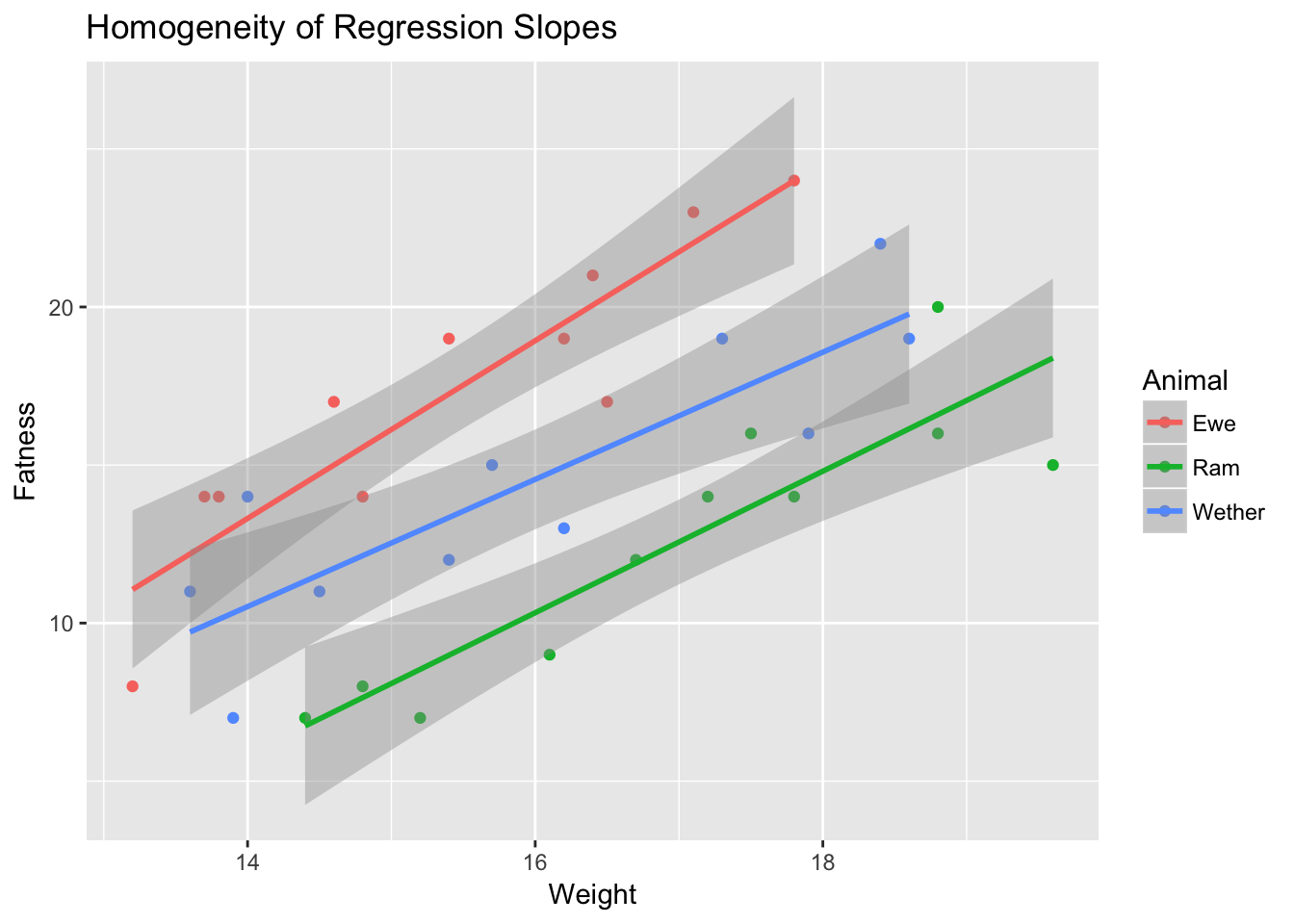
If one of these lines would be pointed downwards, we would have an interaction.