Chapter 15 Repeated Measures ANOVA:
- Repeated measures designs are those in which subjects are tested in each level of the independent variable. 2.The conceptual difference is that repeated measures designs allow for the separate estimation of the influence of individual differences from participant to participant, whereas between subject designs do not. 3.The repeated measures design is more economical and contains more statistical power as compared to its counterpart. 4.The assumptions of the repeated measures ANOVA 5.Power and effect size
The linear model includes two more components, the source of an individual’s performance across the entire study and how an individual interacts with the treatment levels:
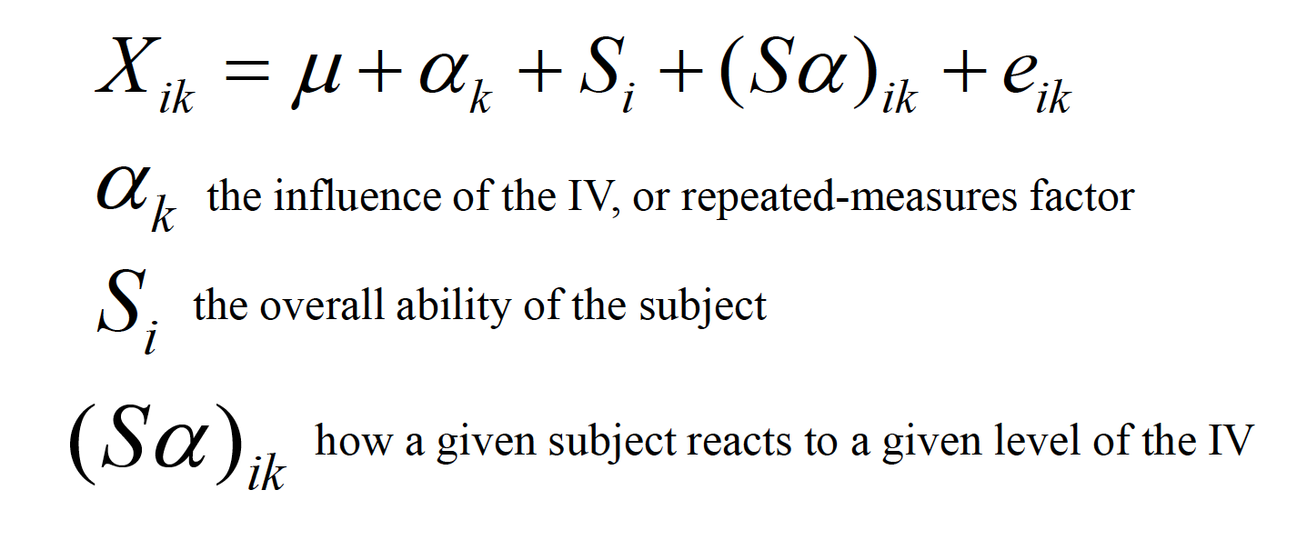
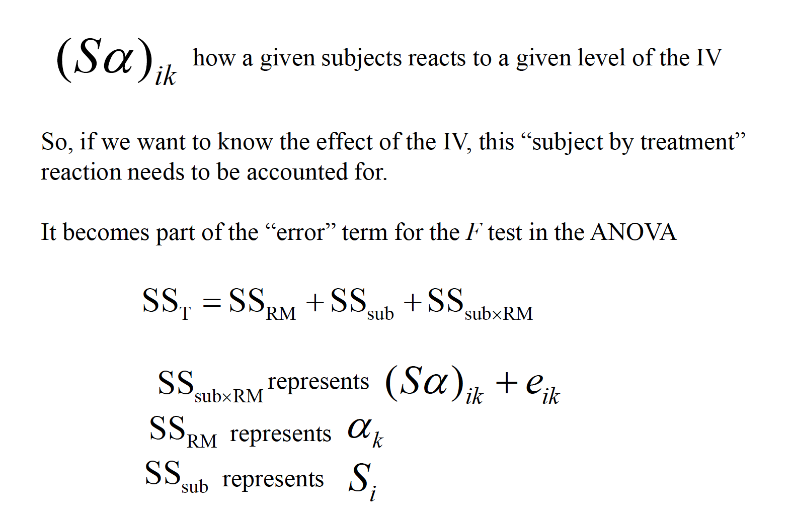
This ability to isolate the source of individual differences allows us to further reduce the error variance (i.e., the denominator of the F ratio).
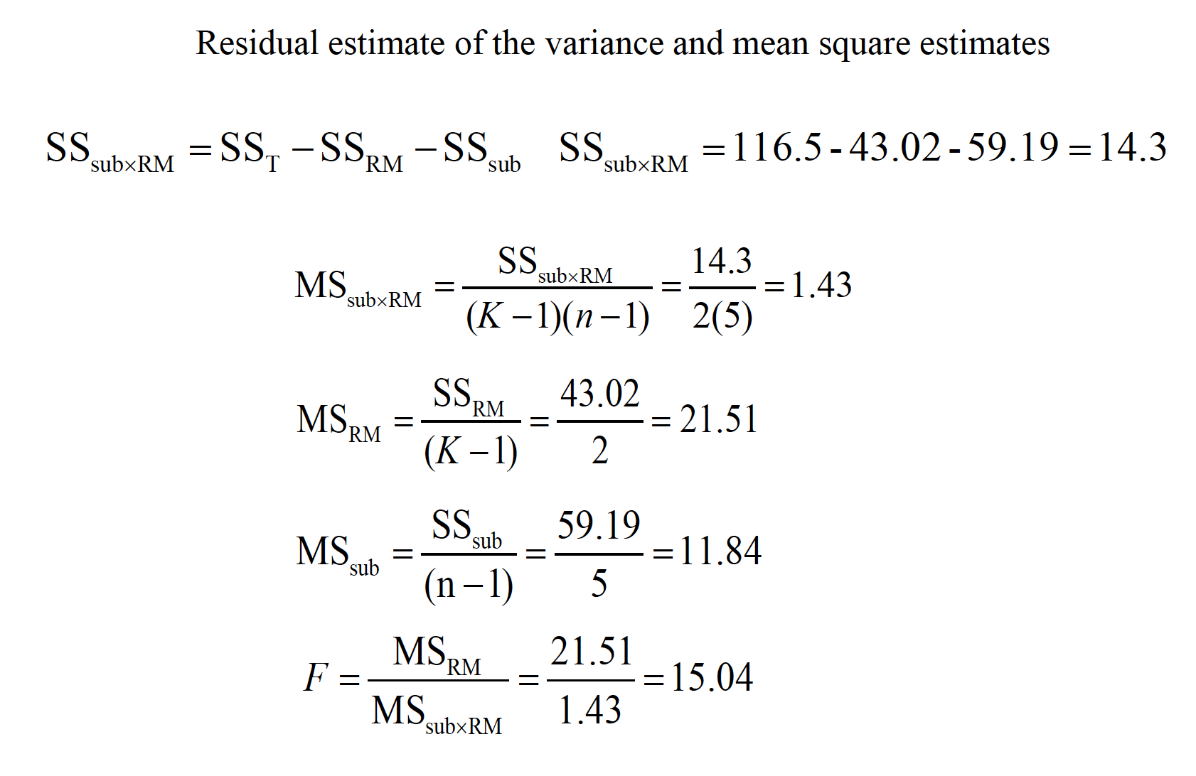
\(F = \frac{MR_{RM}}{MS_{sub x RM}}\)
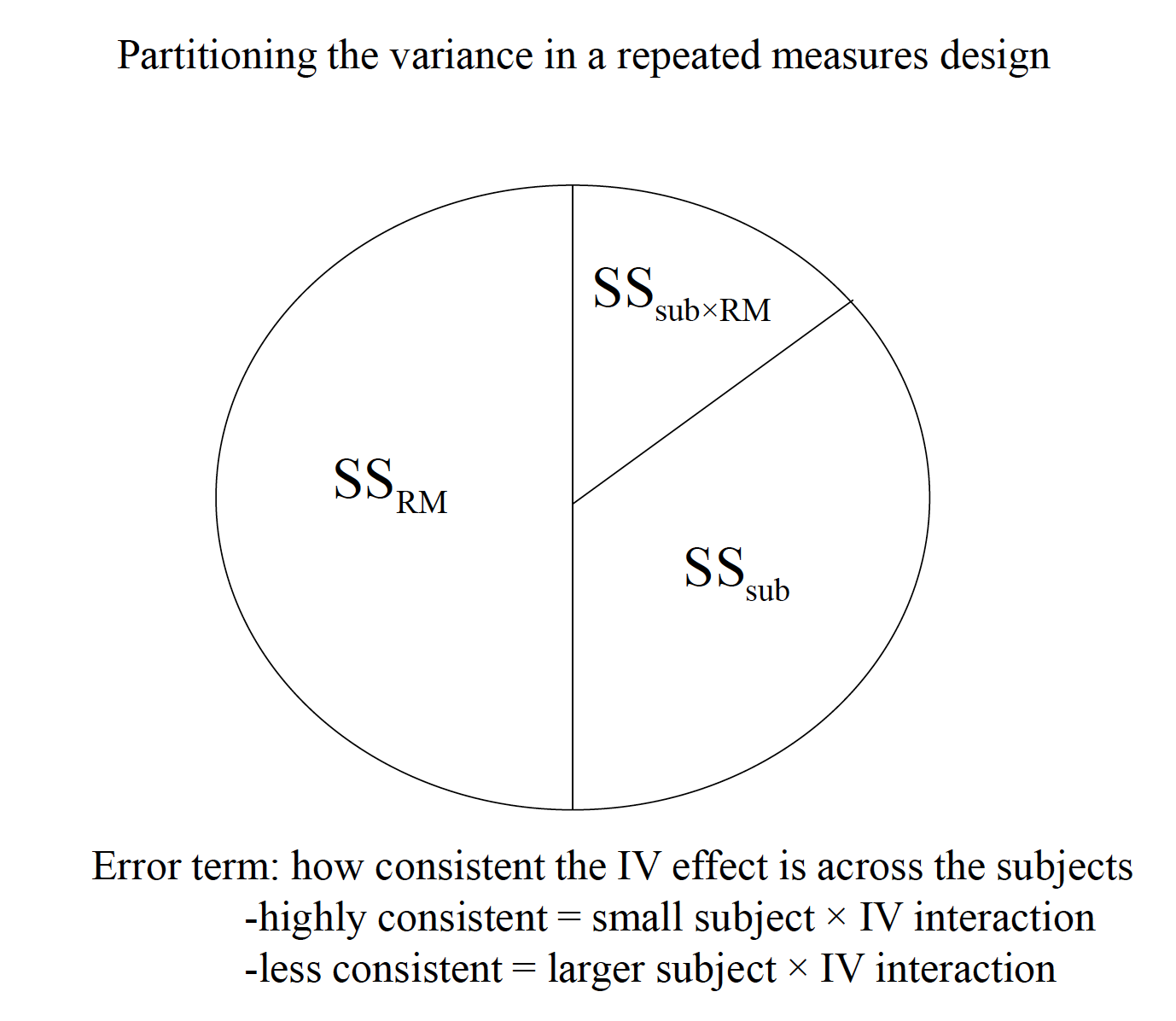
Variability due to subjects is taken into account, but then ignored in the computation of F.
rma
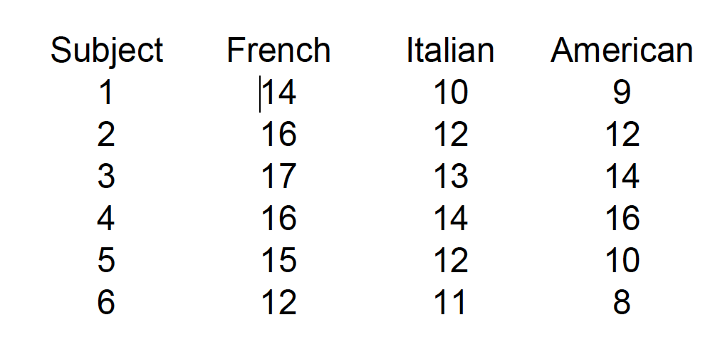
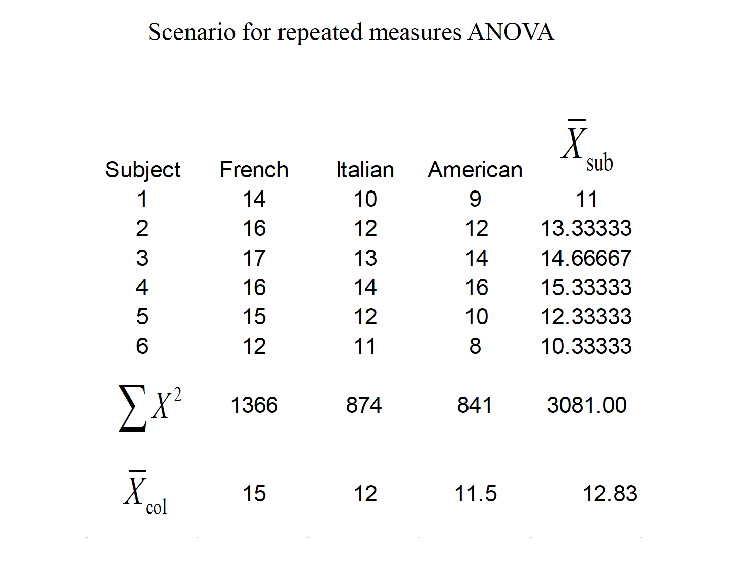
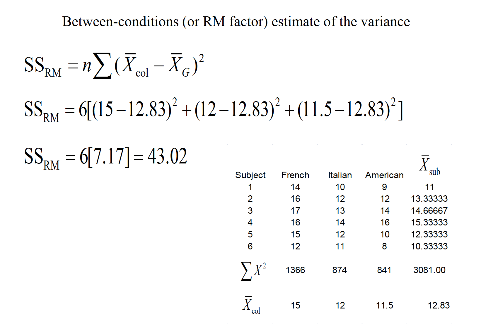
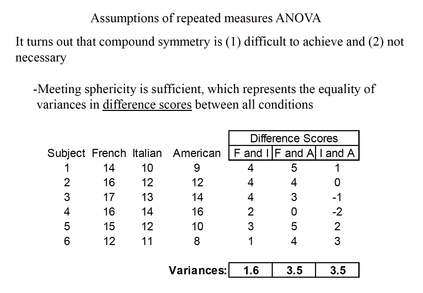
A consumer psychologist is interested in the effect of label information on the perceived quality of wine. Six individuals are asked to rate 3 different wines a scale of 1 to 20, with higher scores being a better quality. The wines were labeled as French, Italian, or American, but the wine was identical across the conditions. The results are shown below:

15.1 Assumptions of RMANOVA
- Sample randomly selected from the population
- The DV is normally distributed in the population
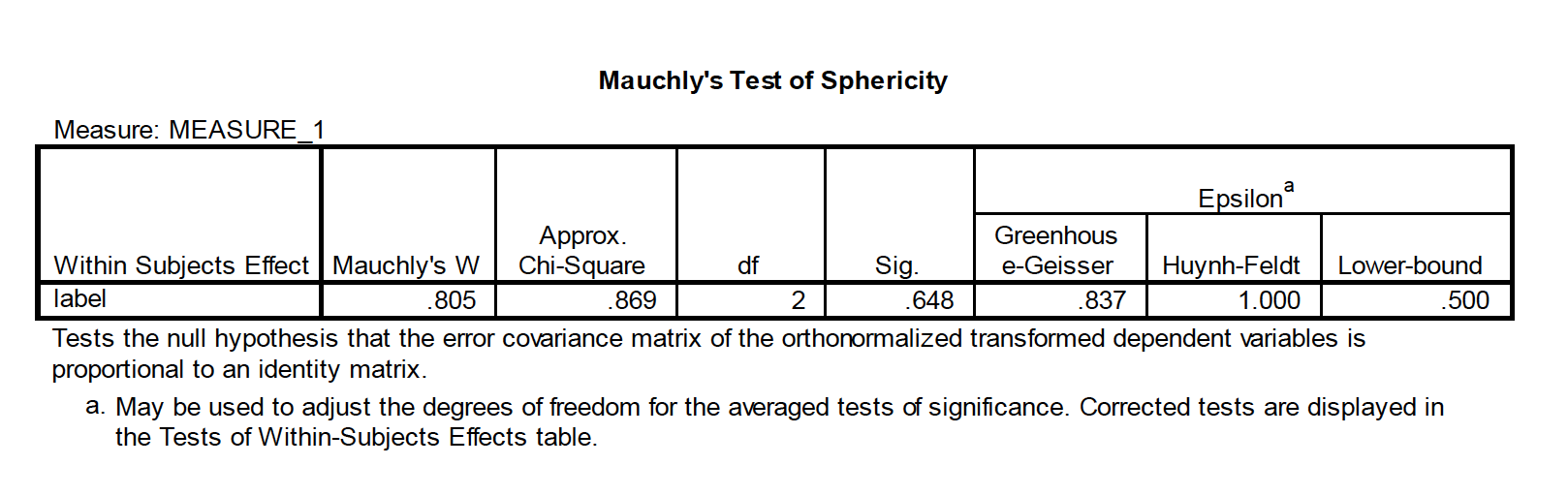
- Sphericity: the variances of difference scores from all possible pairs of conditions are equal
rma
rma
rma
If sphericityis violated, there are several avenues to correct for it that involve applying a correction for the Epsilon value (ε) In SPSS, you’ll see the following in the within-subject ANOVA output: Lower bound correction—this is a change to the critical Fvalue from df= K–1, (n–1)(K–1) to df= 1, n–1. This severelyincreases the critical Fvalue to 6.61 in our case. Huynh & Feldtand Geisser-Greenhouse are corrections to the dfbased on the degree of violation to sphericity, and create more modest corrections to the critical Fvalue. The non-corrected dfare multiplied by the epsilon values for each respective procedure.
If none of the Fs is significant, don’t worry about these corrections—fail to reject the null. If all of the Fs are significant, then reject the null. If one/some of the “corrected” Fs is significant but others are not, then most advocate the Huynh & Feldtcorrection (it’s not as conservative as the lower bound). Field text advocates averaging the G-G and H&F estimates—for a rule of thumb, average the significance values of these estimates
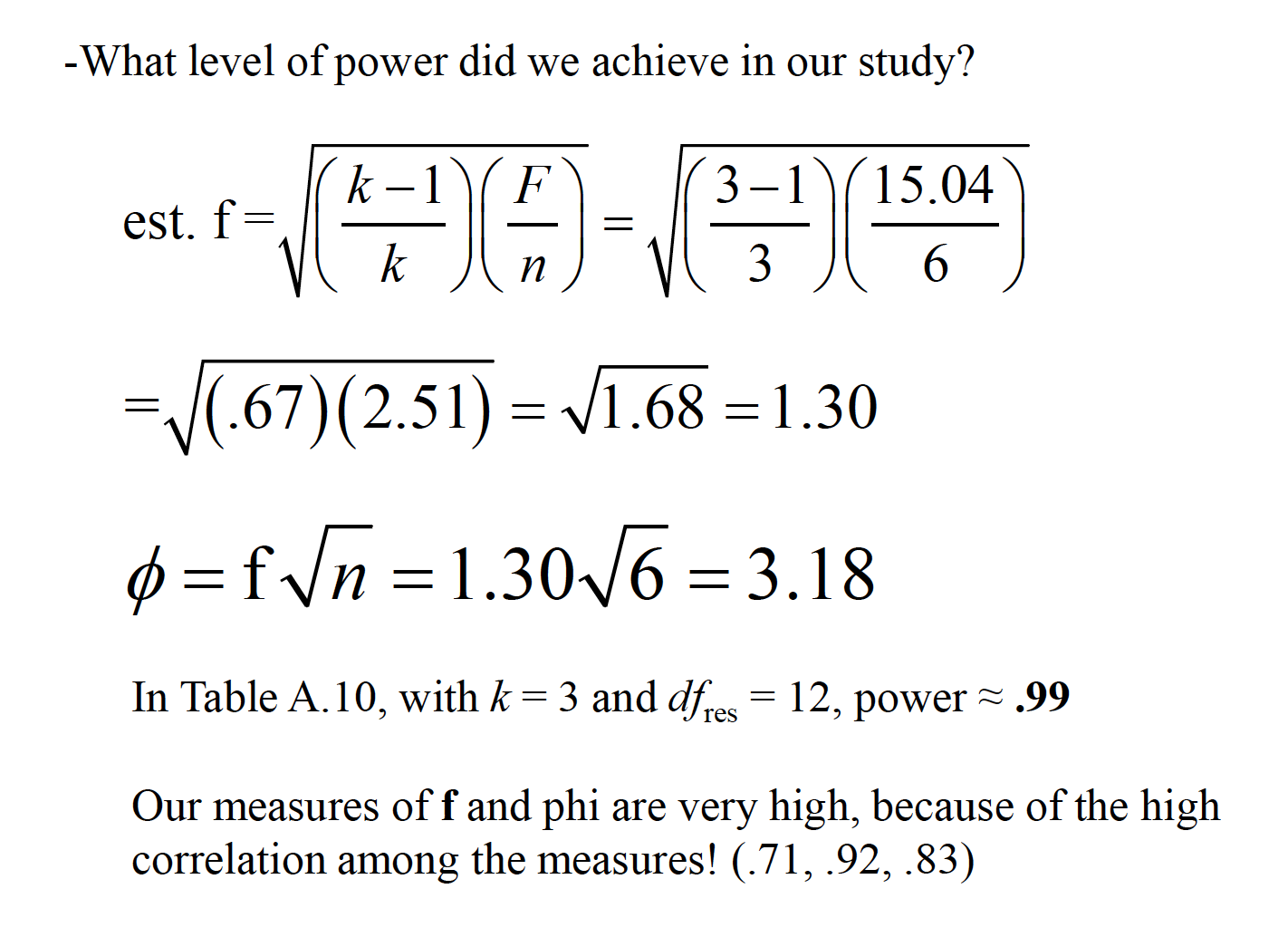
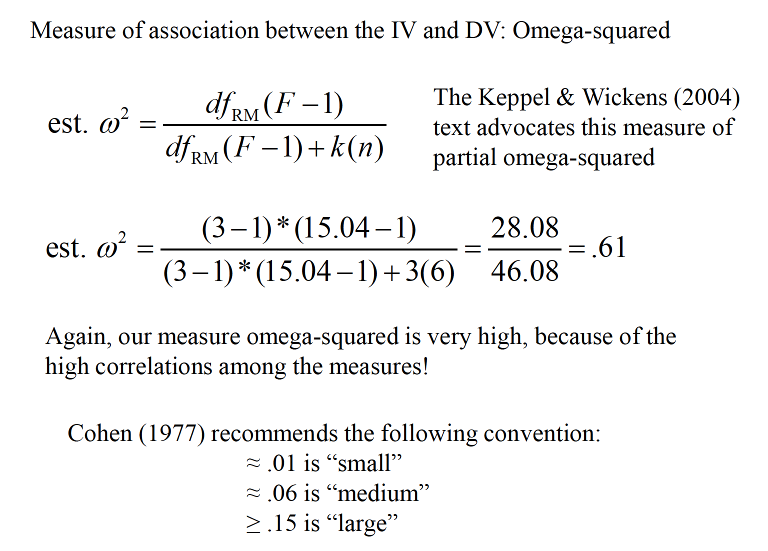
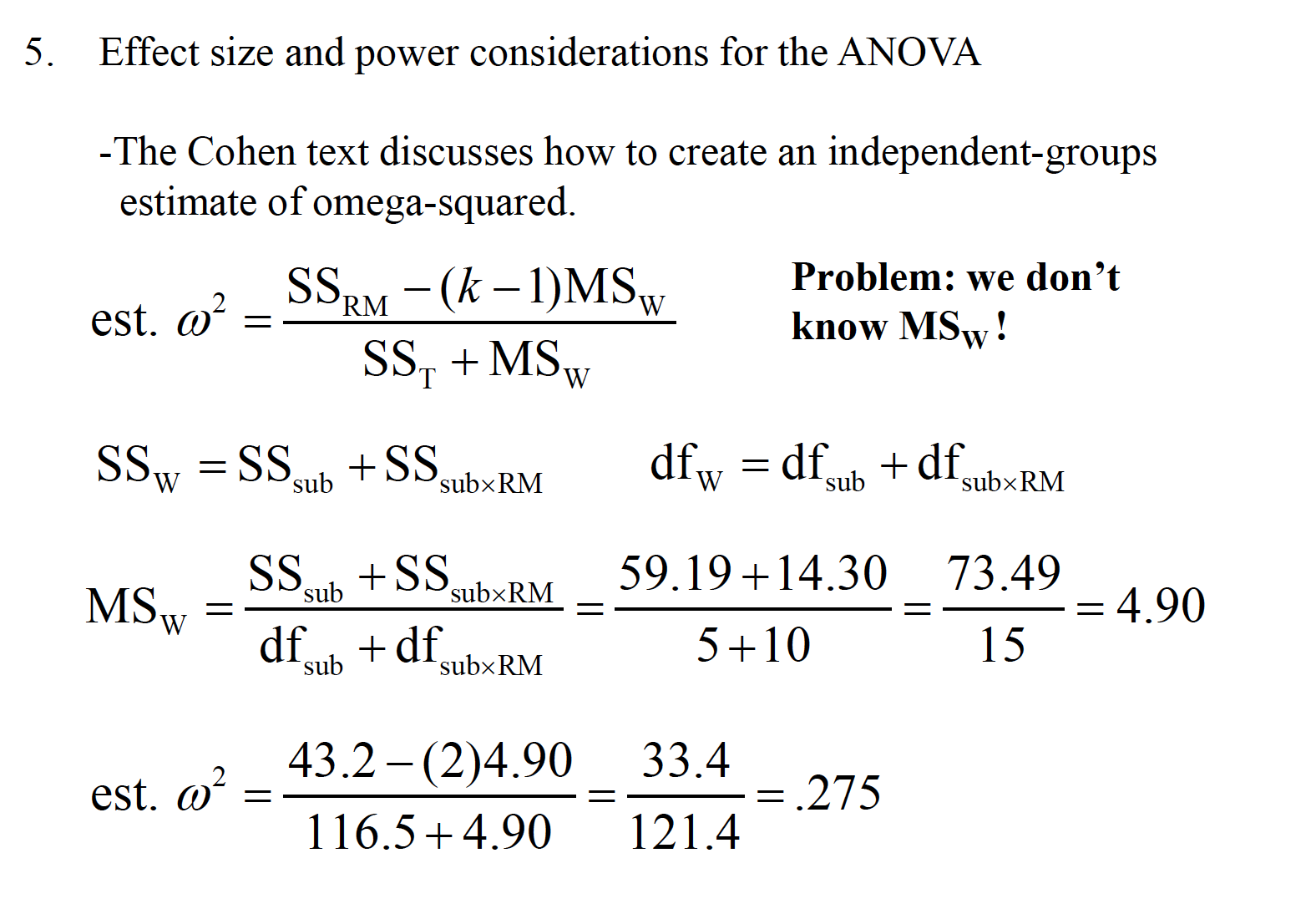
15.2 Effect Size
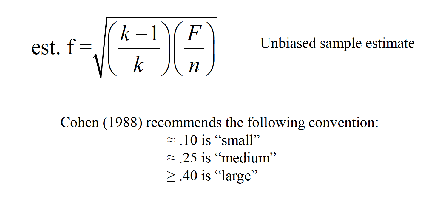
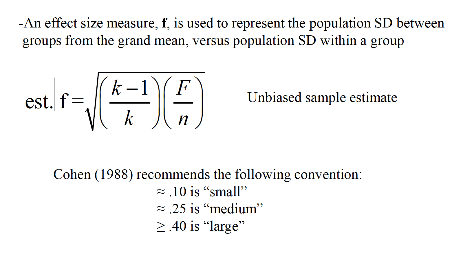
An effect size measure, f, is used to represent the population SD between groups from the grand mean, versus population SD within a group
15.3 DB Notes
Just like regular ANOVA, but now have the assumption of spherecity.
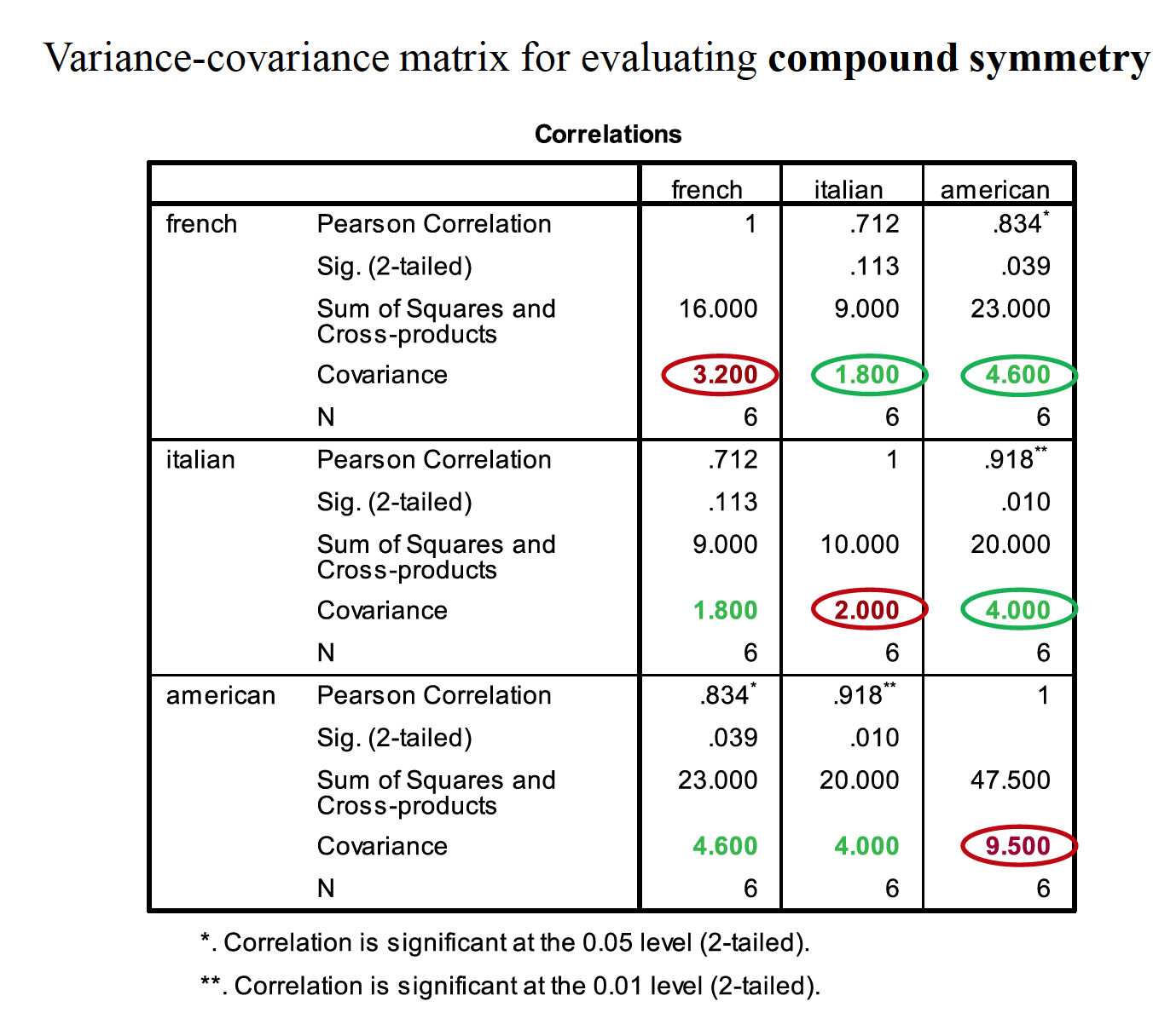
Compound symmetery – variances across conditions are equal and covariances between pairs of conditions are equal. Don’t need this as much in RMANOVA. Spherecity is differences in variation. You do this with Mauchley’s test of sphereicity.
If you violate spherecity, come back here. Can do Greehouse Geisser correction or the Huynh-Feldt corection.
15.3.1 AF Example
participant <- c("P1","P2","P3","P4","P5","P6","P7","P8")
stick_insect <- c(8,9,6,5,8,7,10,12)
kangaroo_testicle <- c(7,5,2,3,4,5,2,6)
fish_eye <- c(1,2,3,1,5,6,7,8)
witch_grub <- c(6,5,8,9,8,7,2,1)
bush <- as.data.frame(cbind(participant, stick_insect, kangaroo_testicle, fish_eye, witch_grub))
Though needs to be long for RMANOVA
##
## Attaching package: 'reshape'
## The following object is masked from 'package:data.table':
##
## meltlongBush <- melt(bush, id = "participant", measured = c("stick_insect", "kangaroo_testicle","fish_eye","witch_grub"))
names(longBush) <- c("Participant","Animal","Retch")
longBush$Animal <- factor(longBush$Animal, labels = c("Stick Insect","Kangaroo","Fish Eye", "Witch"))
longBush## Participant Animal Retch
## 1 P1 Stick Insect 8
## 2 P2 Stick Insect 9
## 3 P3 Stick Insect 6
## 4 P4 Stick Insect 5
## 5 P5 Stick Insect 8
## 6 P6 Stick Insect 7
## 7 P7 Stick Insect 10
## 8 P8 Stick Insect 12
## 9 P1 Kangaroo 7
## 10 P2 Kangaroo 5
## 11 P3 Kangaroo 2
## 12 P4 Kangaroo 3
## 13 P5 Kangaroo 4
## 14 P6 Kangaroo 5
## 15 P7 Kangaroo 2
## 16 P8 Kangaroo 6
## 17 P1 Fish Eye 1
## 18 P2 Fish Eye 2
## 19 P3 Fish Eye 3
## 20 P4 Fish Eye 1
## 21 P5 Fish Eye 5
## 22 P6 Fish Eye 6
## 23 P7 Fish Eye 7
## 24 P8 Fish Eye 8
## 25 P1 Witch 6
## 26 P2 Witch 5
## 27 P3 Witch 8
## 28 P4 Witch 9
## 29 P5 Witch 8
## 30 P6 Witch 7
## 31 P7 Witch 2
## 32 P8 Witch 1PartsVWhole <- c(1,-1,-1,1)
TestVEye <- c(0,-1,1,0)
SticVGrub <- c(-1,0,0,1)
contrasts(longBush$Animal)<-cbind(PartsVWhole,TestVEye,SticVGrub)
longBush$Animal## [1] Stick Insect Stick Insect Stick Insect Stick Insect Stick Insect
## [6] Stick Insect Stick Insect Stick Insect Kangaroo Kangaroo
## [11] Kangaroo Kangaroo Kangaroo Kangaroo Kangaroo
## [16] Kangaroo Fish Eye Fish Eye Fish Eye Fish Eye
## [21] Fish Eye Fish Eye Fish Eye Fish Eye Witch
## [26] Witch Witch Witch Witch Witch
## [31] Witch Witch
## attr(,"contrasts")
## PartsVWhole TestVEye SticVGrub
## Stick Insect 1 0 -1
## Kangaroo -1 -1 0
## Fish Eye -1 1 0
## Witch 1 0 1
## Levels: Stick Insect Kangaroo Fish Eye WitchRunning It
THIS IS BROKEN
## 'data.frame':    32 obs. of  3 variables:
##  $ Participant: Factor w/ 8 levels "P1","P2","P3",..: 1 2 3 4 5 6 7 8 1 2 ...
##  $ Animal     : Factor w/ 4 levels "Stick Insect",..: 1 1 1 1 1 1 1 1 2 2 ...
##   ..- attr(*, "contrasts")= num [1:4, 1:3] 1 -1 -1 1 0 -1 1 0 -1 0 ...
##   .. ..- attr(*, "dimnames")=List of 2
##   .. .. ..$ : chr  "Stick Insect" "Kangaroo" "Fish Eye" "Witch"
##   .. .. ..$ : chr  "PartsVWhole" "TestVEye" "SticVGrub"
##  $ Retch      : Factor w/ 11 levels "10","12","5",..: 6 7 4 3 6 5 1 2 5 3 ...